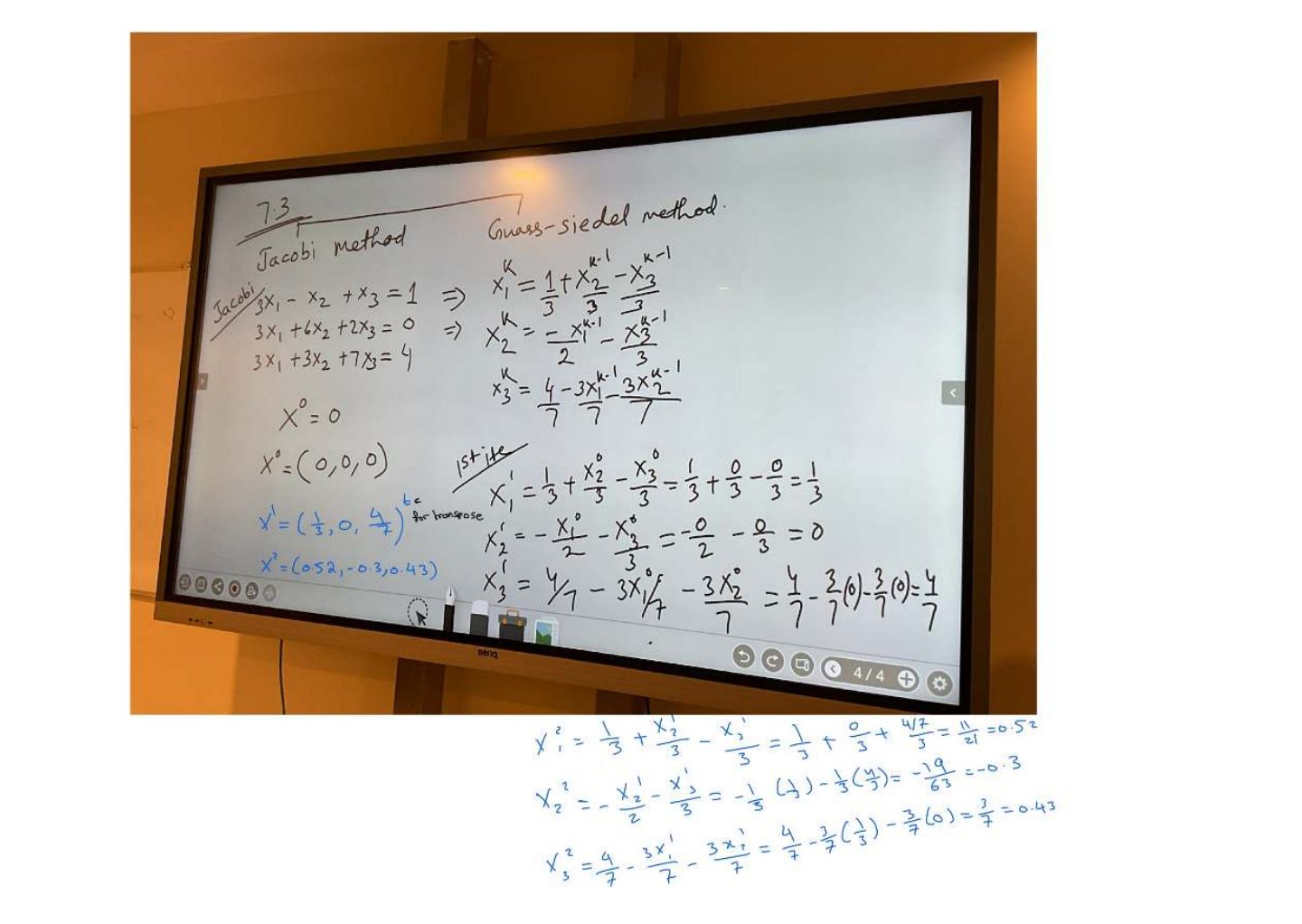
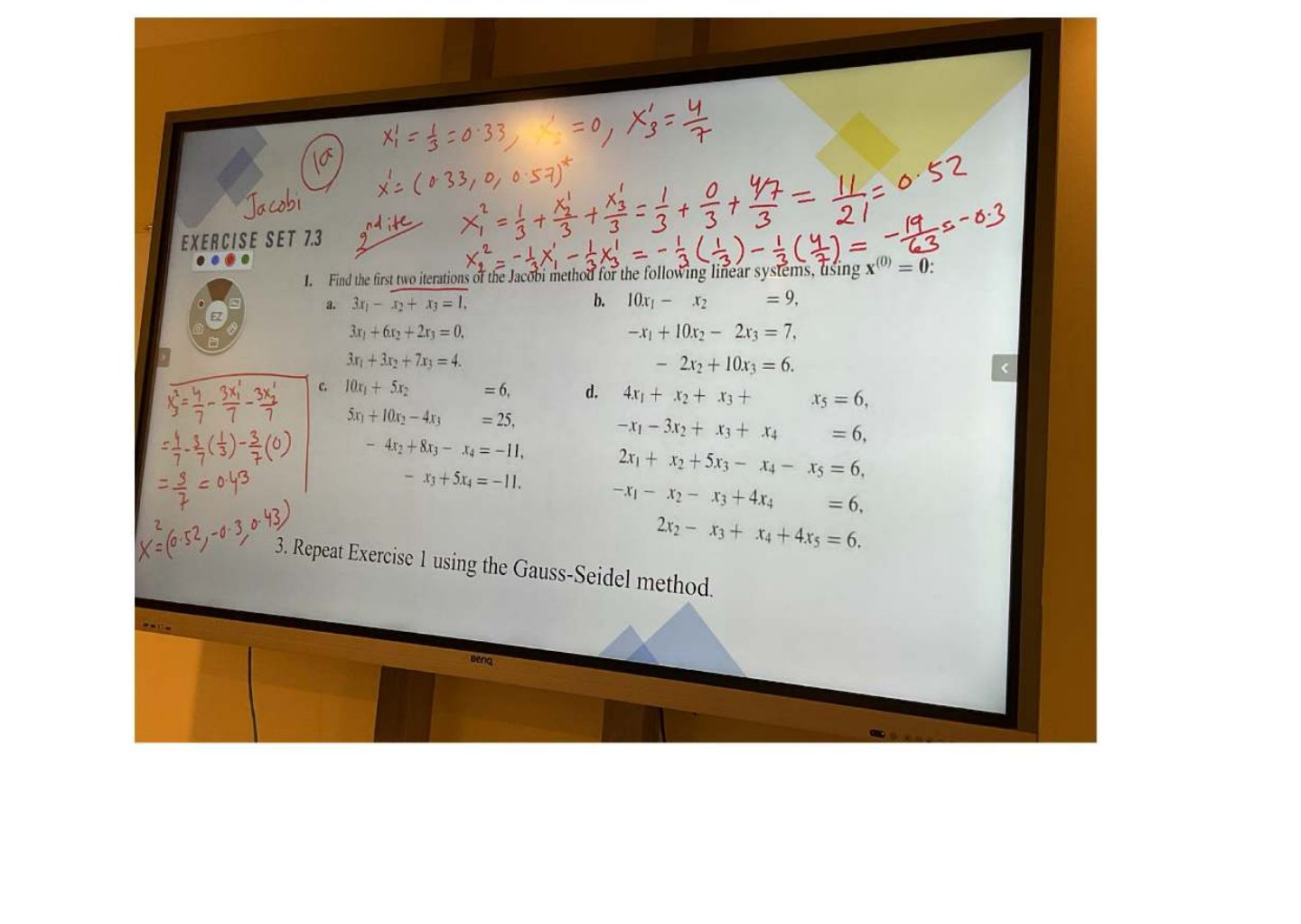
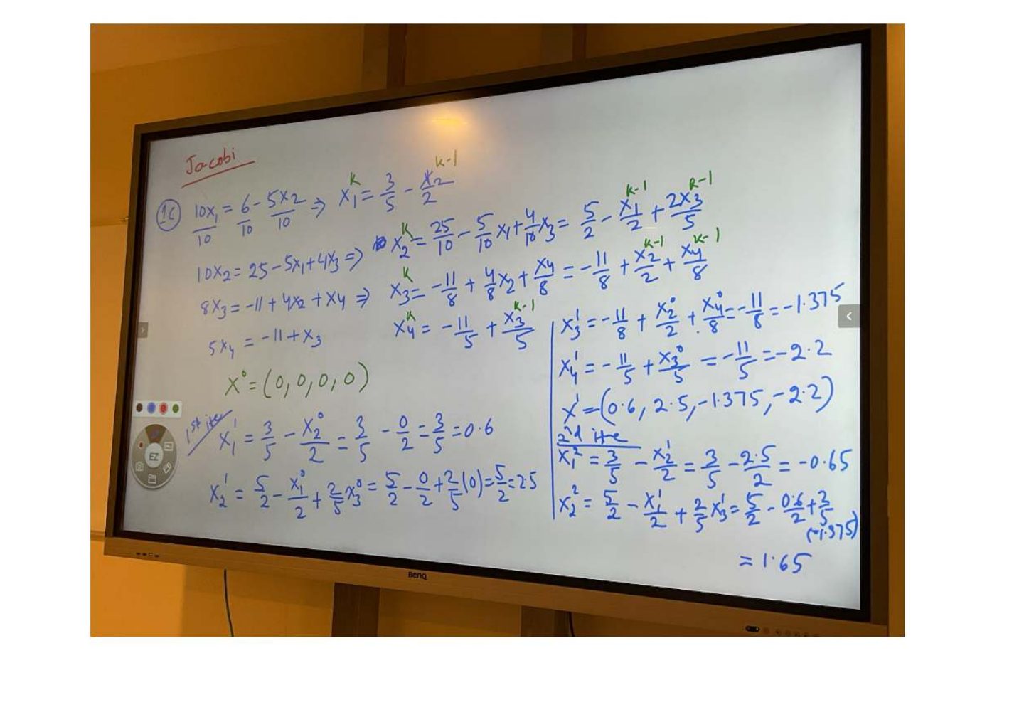
One Gauss–Seidel step for 10x − y = 9, −x + 10y = 9 from (0, 0).
Compare with the model answer
x = (9 + 0)/10 = 0.9; y = (9 + 0.9)/10 = 0.99.
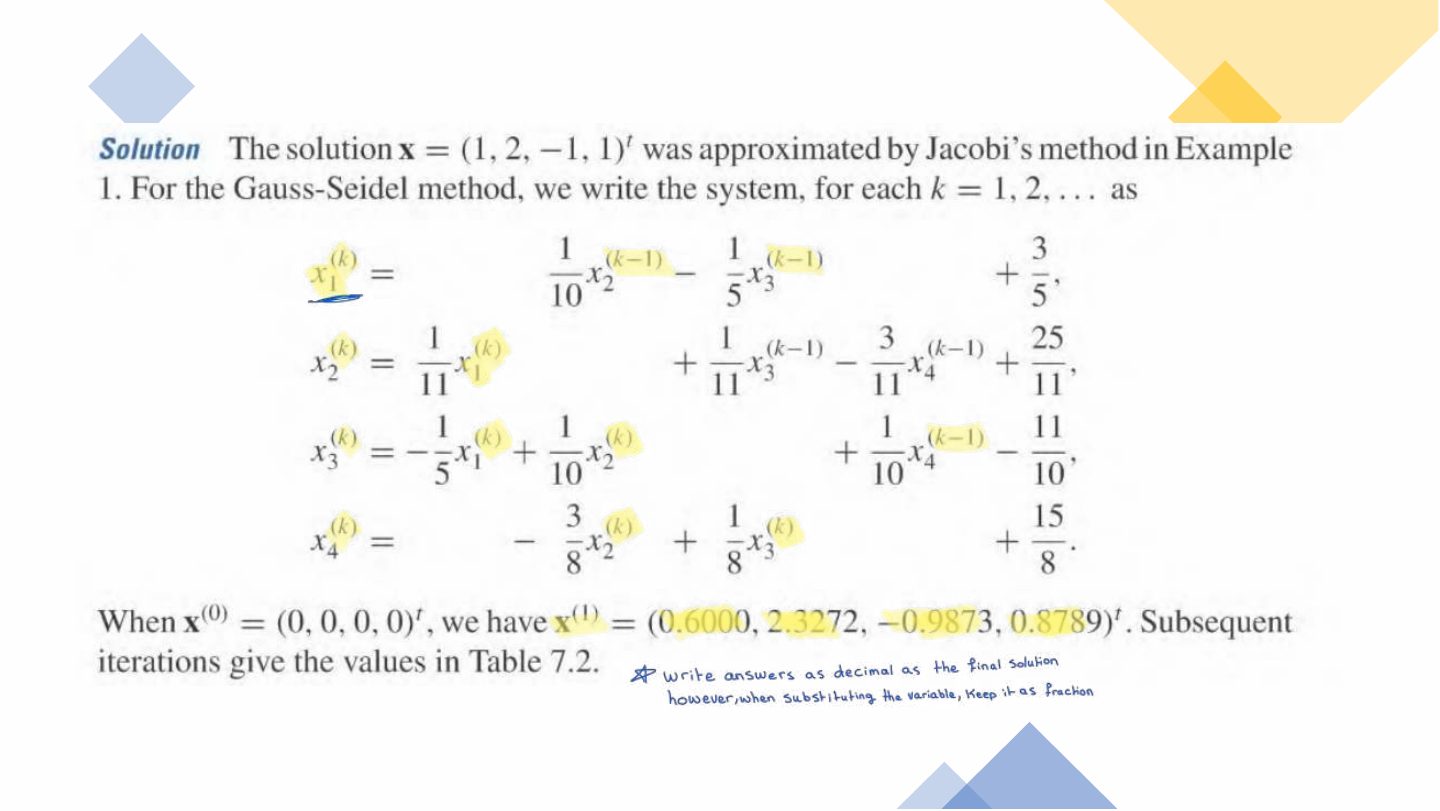
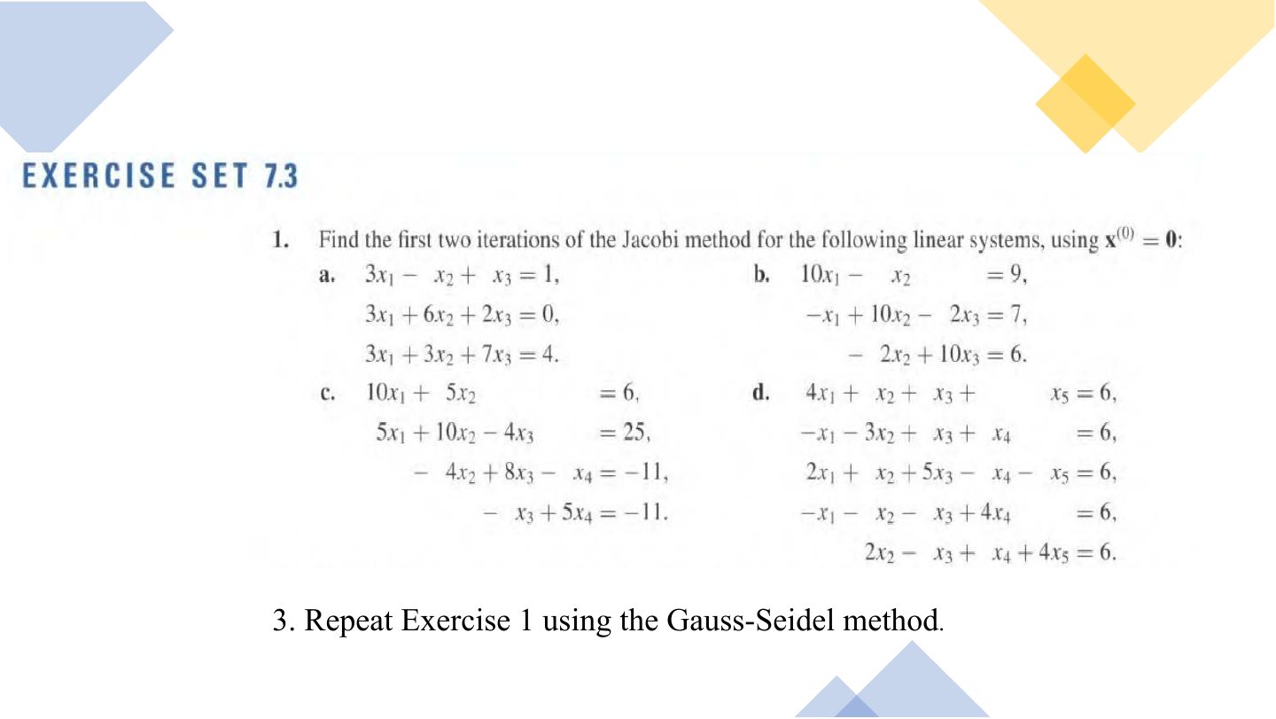
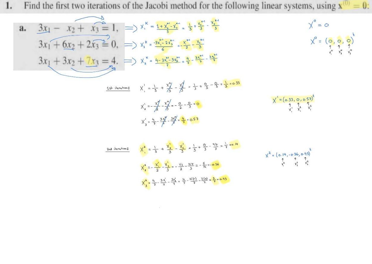
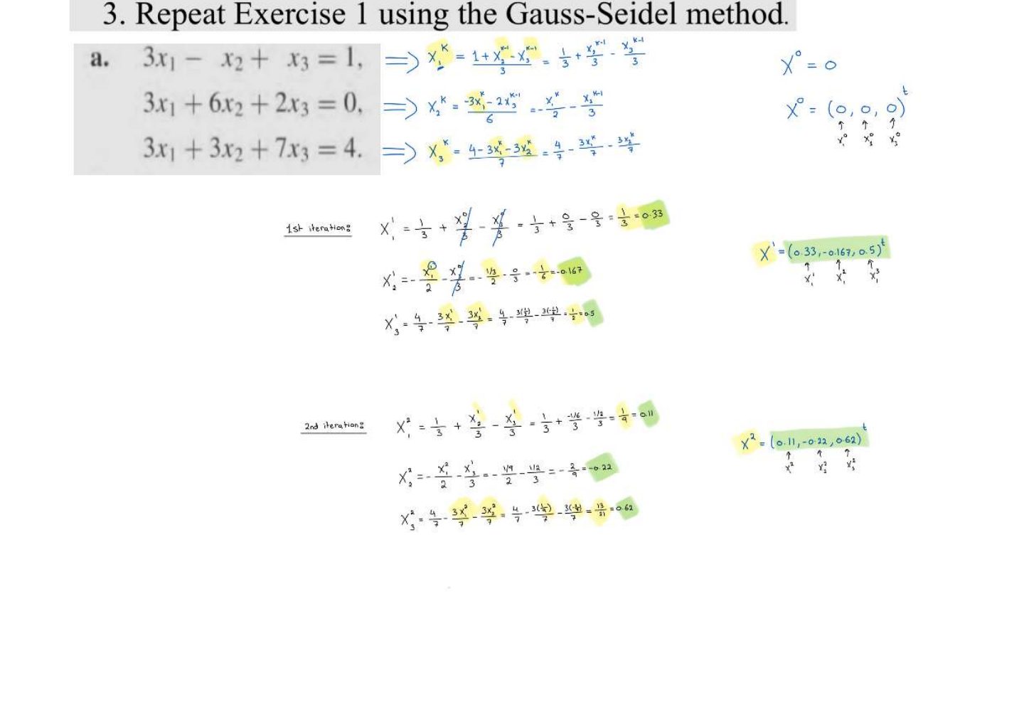
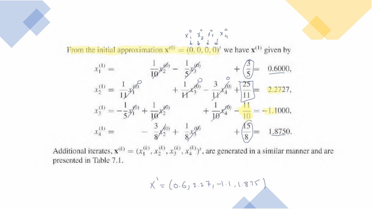
The Jacobi and Gauss–Seidel iterative techniques and their convergence.
Every original slide is shown unchanged. Yellow marks on a slide point to a numbered note: hover or tap a mark to jump to its note, and hover a note to see its marks. Questions tagged Past exam appeared on a real paper; Prediction questions are likely angles, not confirmed. Pick an answer to each question: a wrong pick tells you why it is wrong, so you can try again.
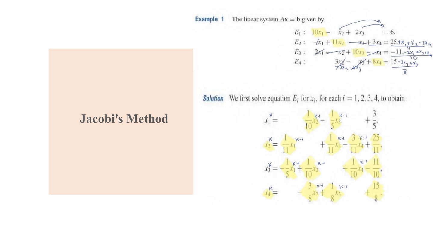
Jacobi: xᵢ⁽ᵏ⁾ = (bᵢ − Σ_{j≠i} aᵢⱼxⱼ⁽ᵏ⁻¹⁾)/aᵢᵢ (all old values).
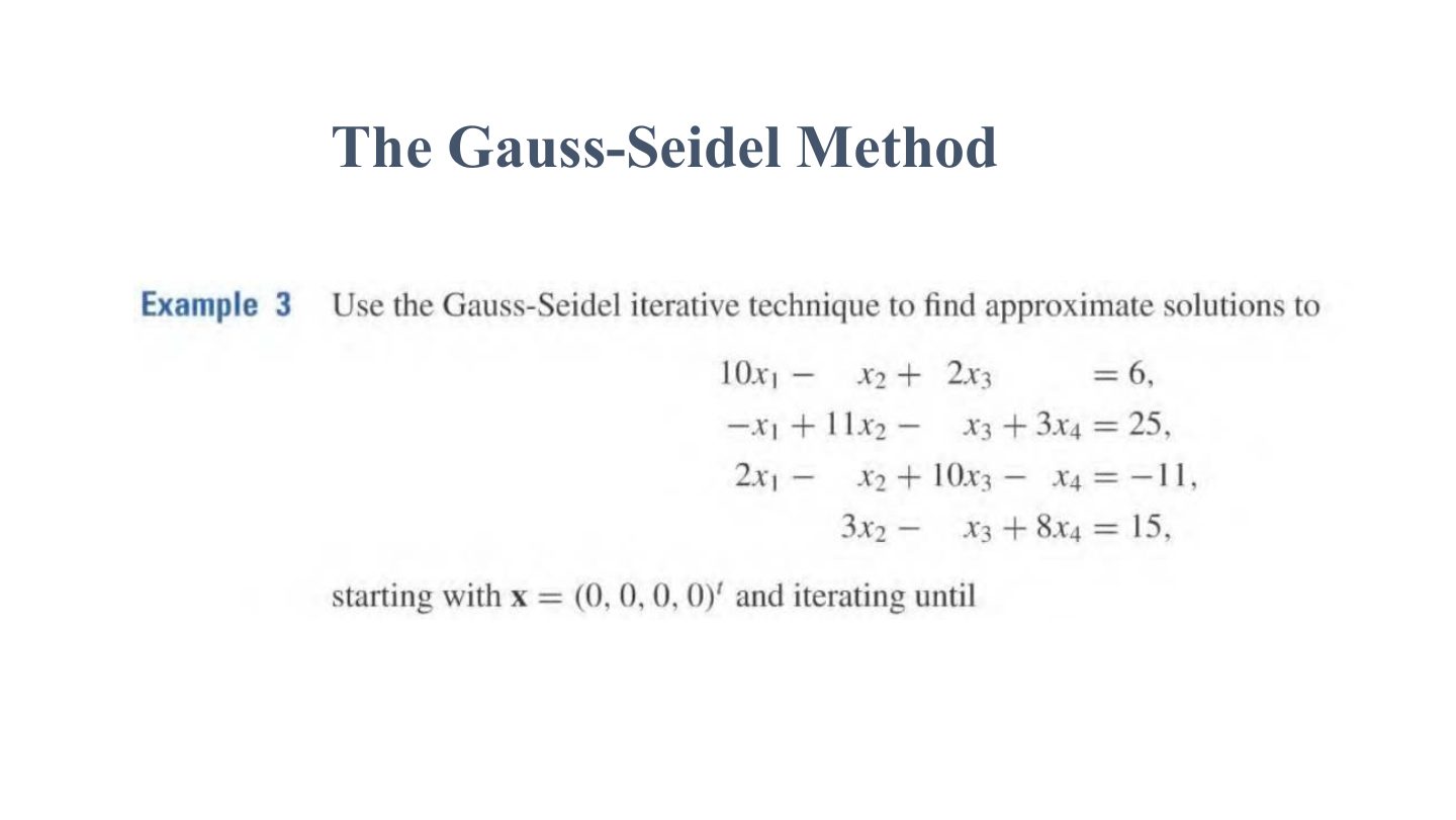
Gauss–Seidel: uses the newest values as soon as they are computed; usually faster. Both converge if A is strictly diagonally dominant.
Memory trick Jacobi = old values; Gauss–Seidel = newest values.
One Gauss–Seidel step for 10x − y = 9, −x + 10y = 9 from (0, 0).
x = (9 + 0)/10 = 0.9; y = (9 + 0.9)/10 = 0.99.