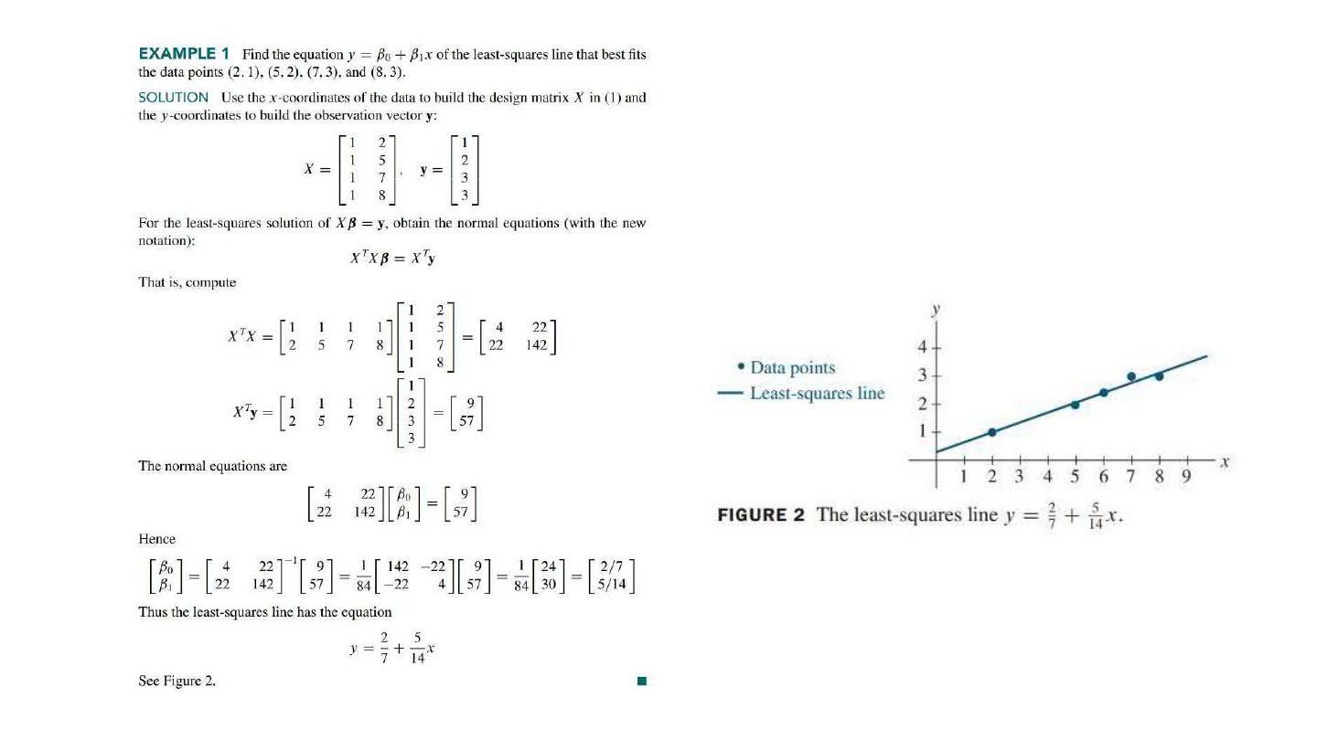
Set up the design matrix for fitting y = β₀ + β₁x to points (2, 1), (5, 2), (7, 3).
Compare with the model answer
X = [[1, 2], [1, 5], [1, 7]], y = (1, 2, 3); solve XᵀXβ = Xᵀy.
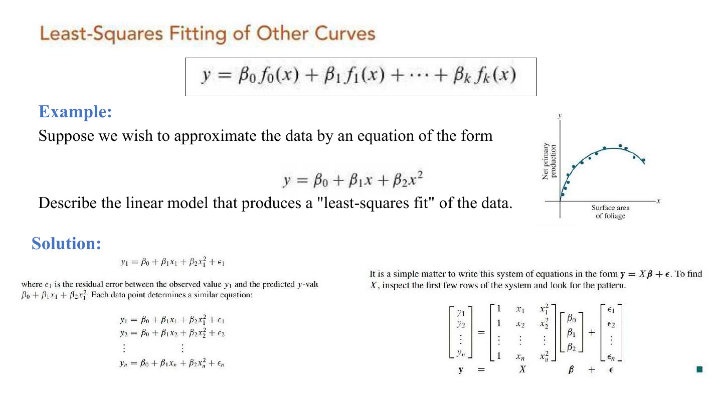
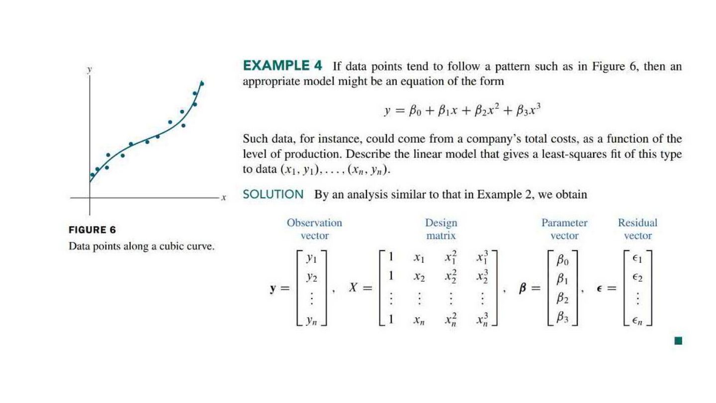
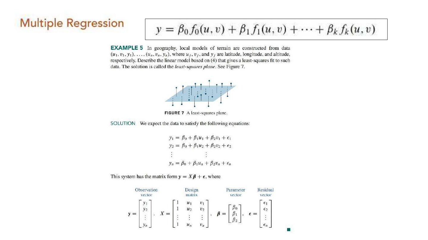
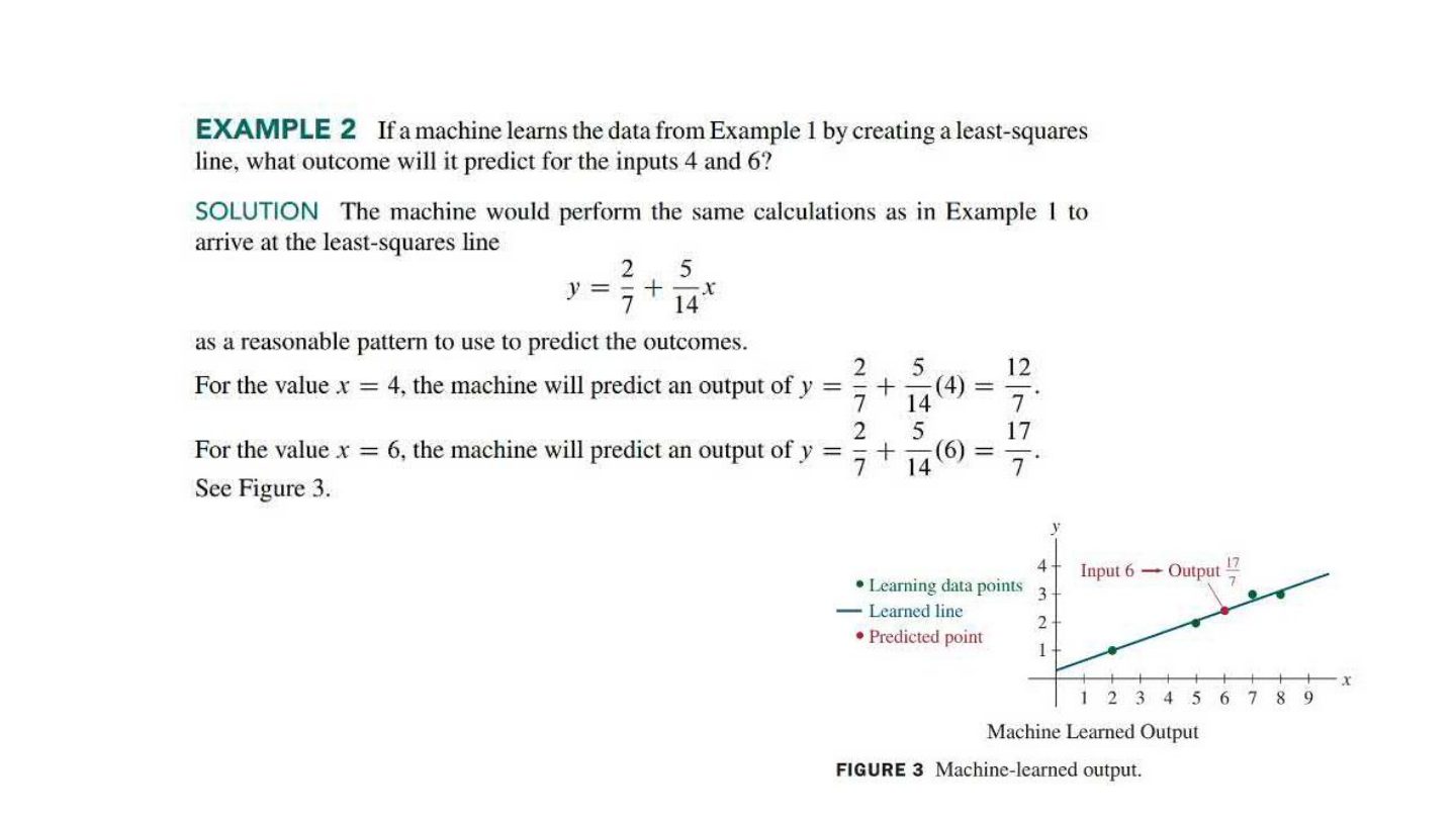
Regression as least squares: the design matrix X, parameter vector β and observation vector y, the least-squares line y = β₀ + β₁x, residuals, and fitting other curves.
Every original slide is shown unchanged. Yellow marks on a slide point to a numbered note: hover or tap a mark to jump to its note, and hover a note to see its marks. Questions tagged Past exam appeared on a real paper; Prediction questions are likely angles, not confirmed. Pick an answer to each question: a wrong pick tells you why it is wrong, so you can try again.
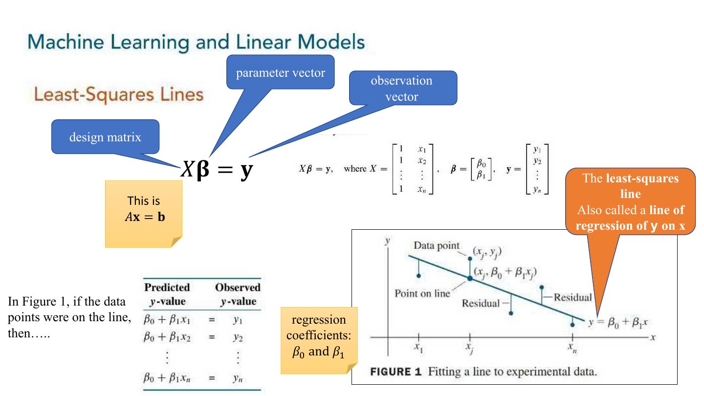
Linear model y = Xβ + ε. Least-squares line: X has a column of 1s and a column of x values; solve XᵀXβ = Xᵀy.
Set up the design matrix for fitting y = β₀ + β₁x to points (2, 1), (5, 2), (7, 3).
X = [[1, 2], [1, 5], [1, 7]], y = (1, 2, 3); solve XᵀXβ = Xᵀy.
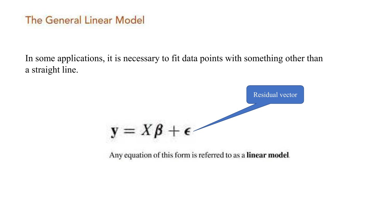
Other curves (e.g. y = β₀ + β₁x + β₂x²) are still LINEAR in the parameters: add a column for x².