Filling and updating routing tables by finding best paths is called:
Network Layer: Routing of Packets
How routers fill their tables: the internet as a weighted graph, static vs. dynamic routing, host-specific, network-specific and default routes, forwarding with masks (longest mask first), distance-vector (Bellman-Ford) vs. link-state (Dijkstra) routing, and autonomous systems with interior (RIP, OSPF, EIGRP) and exterior (BGP) protocols. Rebuilt from the highlighted copy of the deck until a clean one is uploaded, so a few figures show light highlighting.
How to read this page
Every original slide is shown unchanged. Yellow marks on a slide point to a numbered note: hover or tap a mark to jump to its note, and hover a note to see its marks. Questions tagged Past exam appeared on a real paper; Prediction questions are likely angles, not confirmed. Pick an answer to each question: a wrong pick tells you why it is wrong, so you can try again.
All 36 slides
- 1 Network Layer: Routing of Packets
- 2 Chapter 8: Outline
- 3 Routing (IP routing)
- 4 8-1 INTRODUCTION
- 5 8.1.1 General Idea
- 6 An Internet as a Graph
- 7 An internet and its graphical representation (Figure 8.1)
- 8 Graph representation of a network
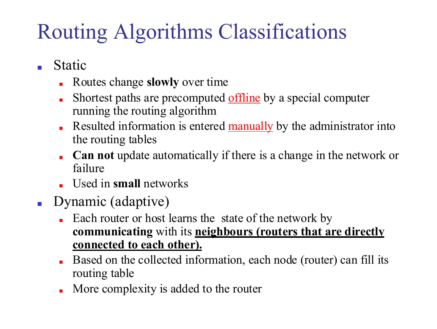
- 9 Routing Algorithms Classifications
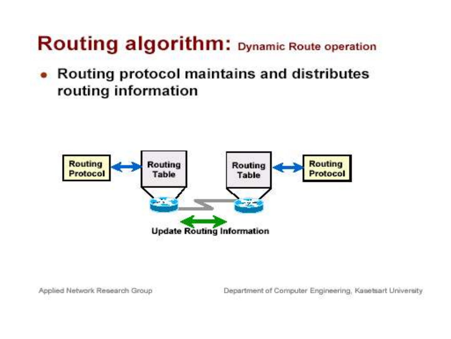
- 10 Routing algorithm: dynamic route operation
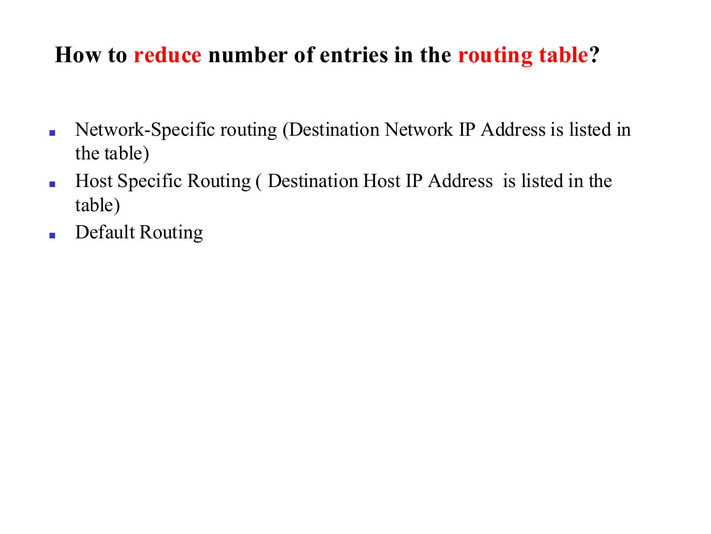
- 11 How to reduce number of entries in the routing table?
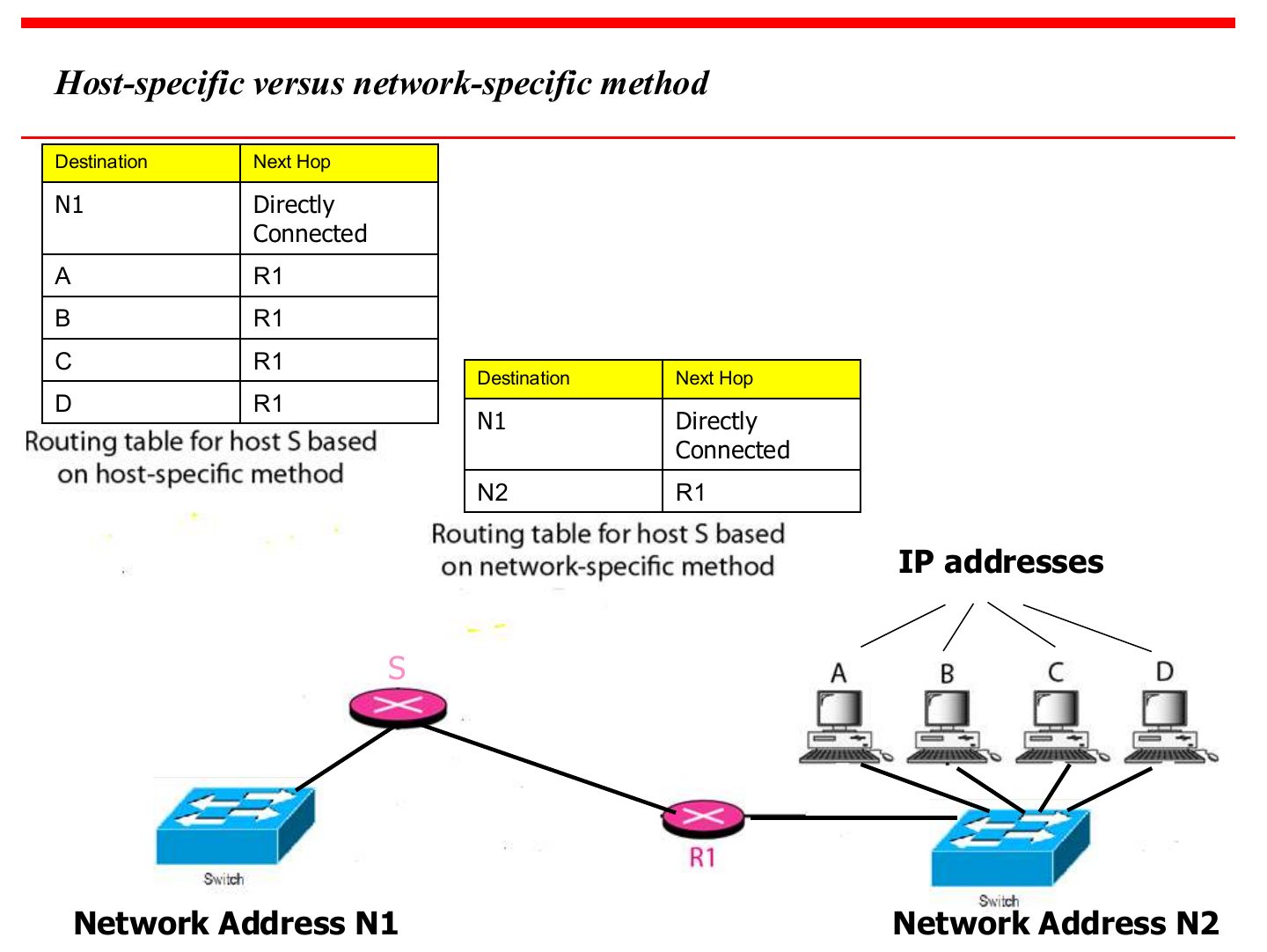
- 12 Host-specific versus network-specific method
- 13 Default Route
- 14 Forwarding of IP packets
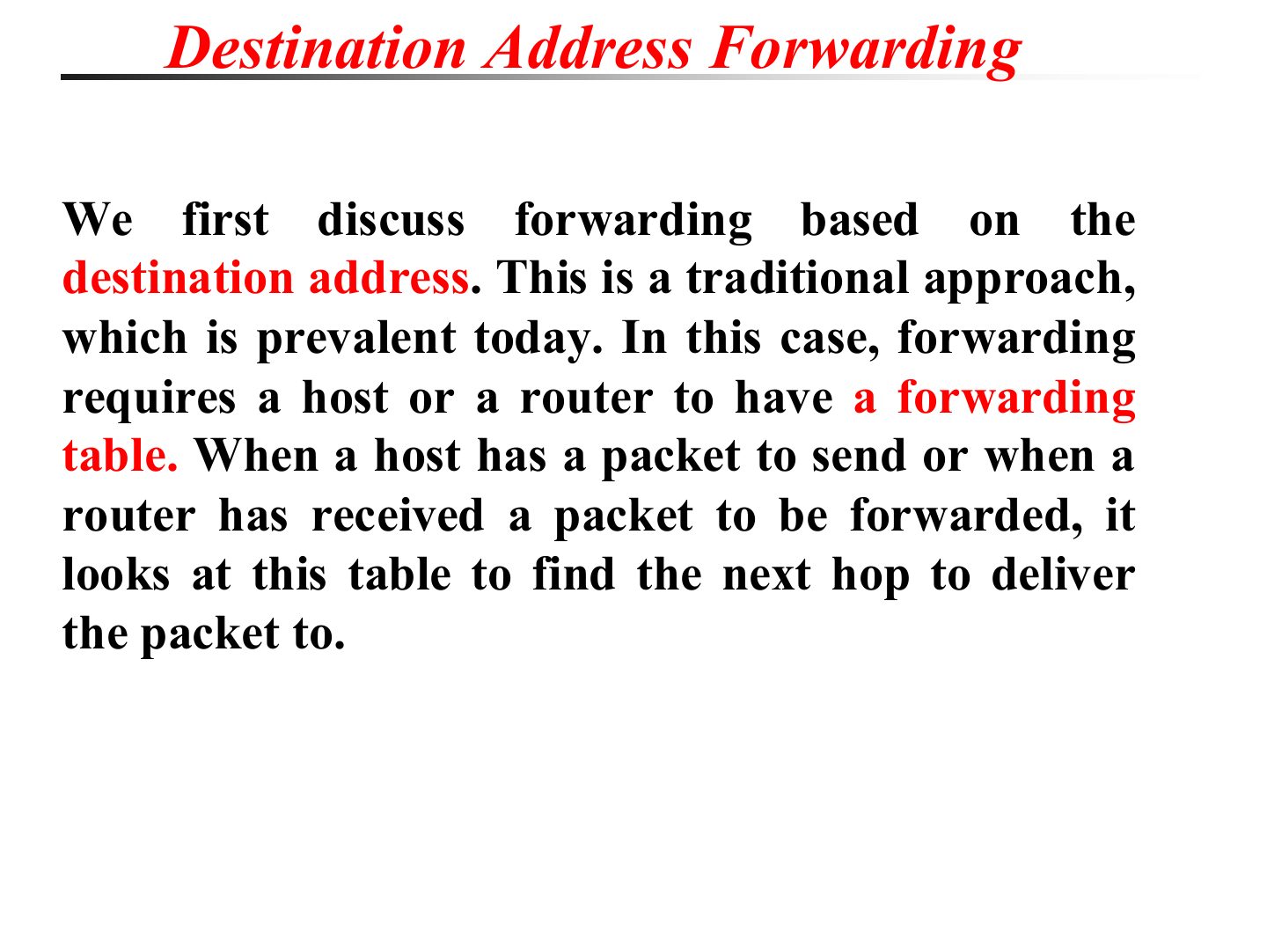
- 15 Destination Address Forwarding
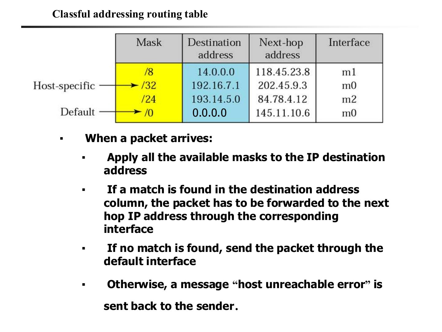
- 16 Classful addressing routing table
- 17 Example
- 18 Example
- 19 Example
- 20 Example: router R1’s networks
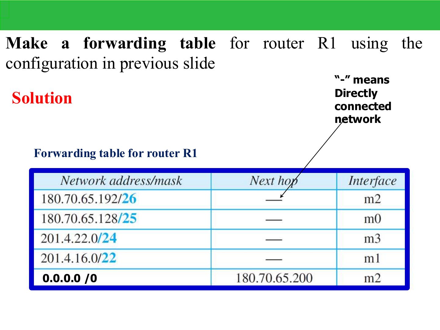
- 21 Forwarding table for router R1
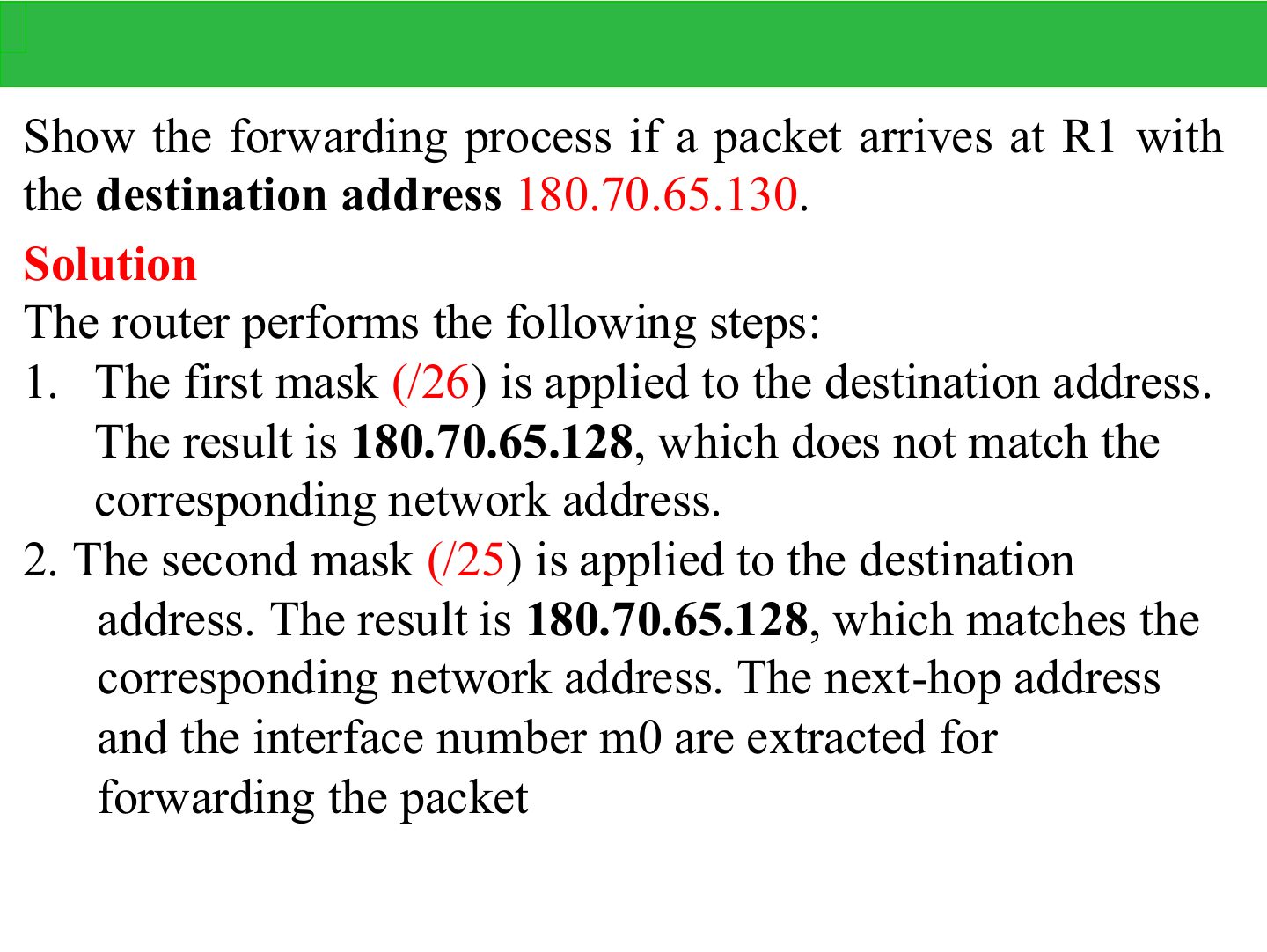
- 22 Show the forwarding process if a packet arrives at R1 with the destination address 180.70.65.130.
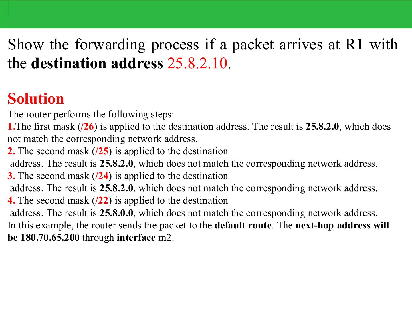
- 23 Show the forwarding process if a packet arrives at R1 with the destination address 25.8.2.10.
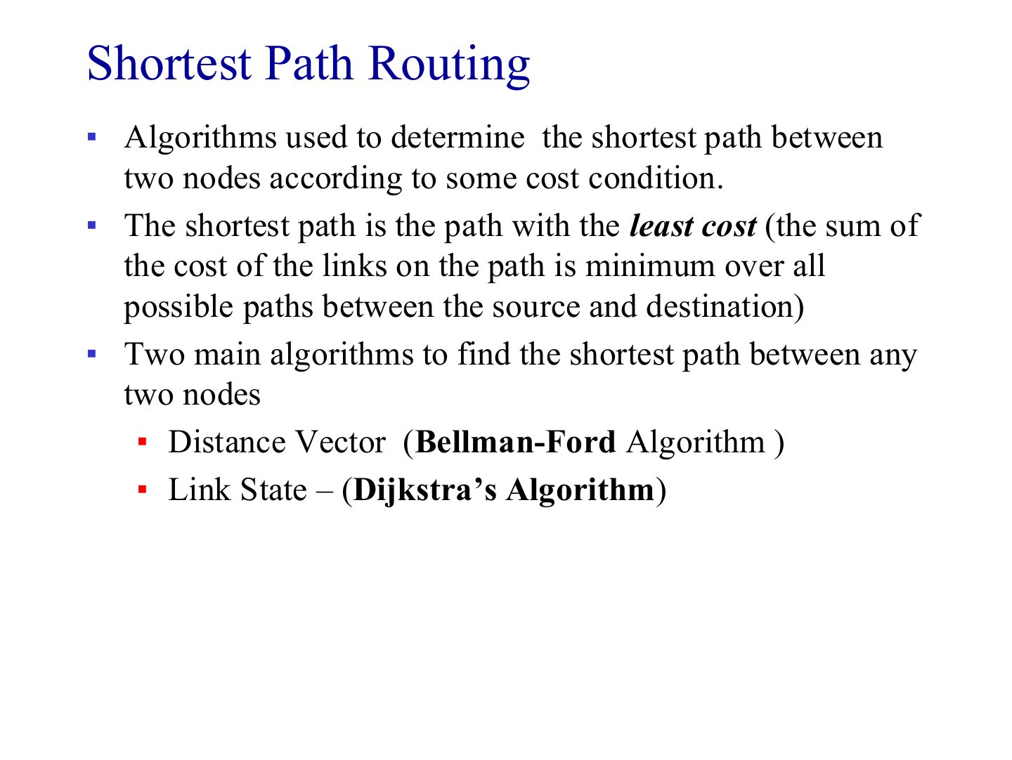
- 24 Shortest Path Routing
- 25 Distance Vector (DV) Routing
- 26 The first-round distance vectors
- 27 Updating distance vectors (node B)
- 28 The distance vector corresponding to a tree
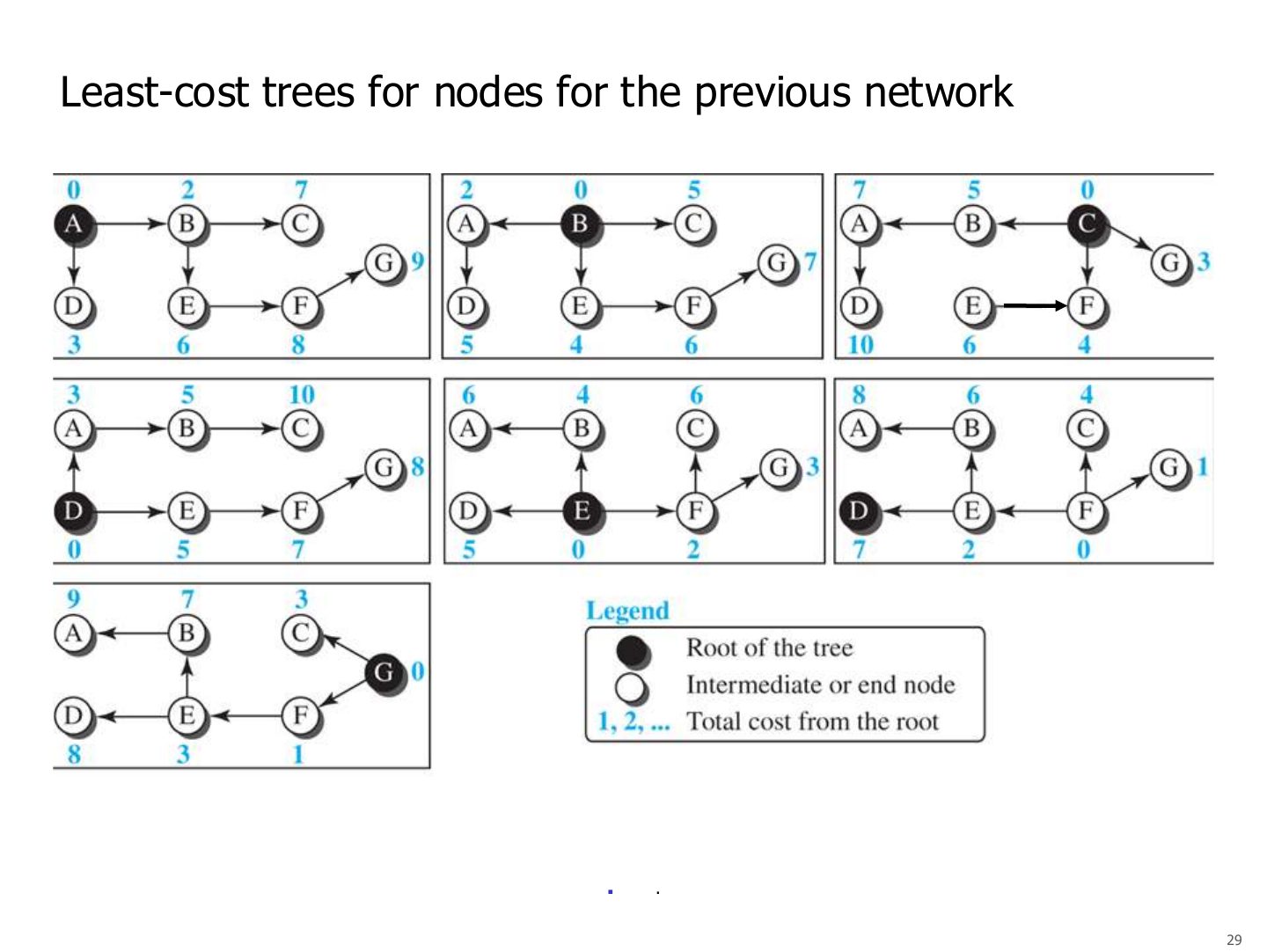
- 29 Least-cost trees for nodes for the previous network
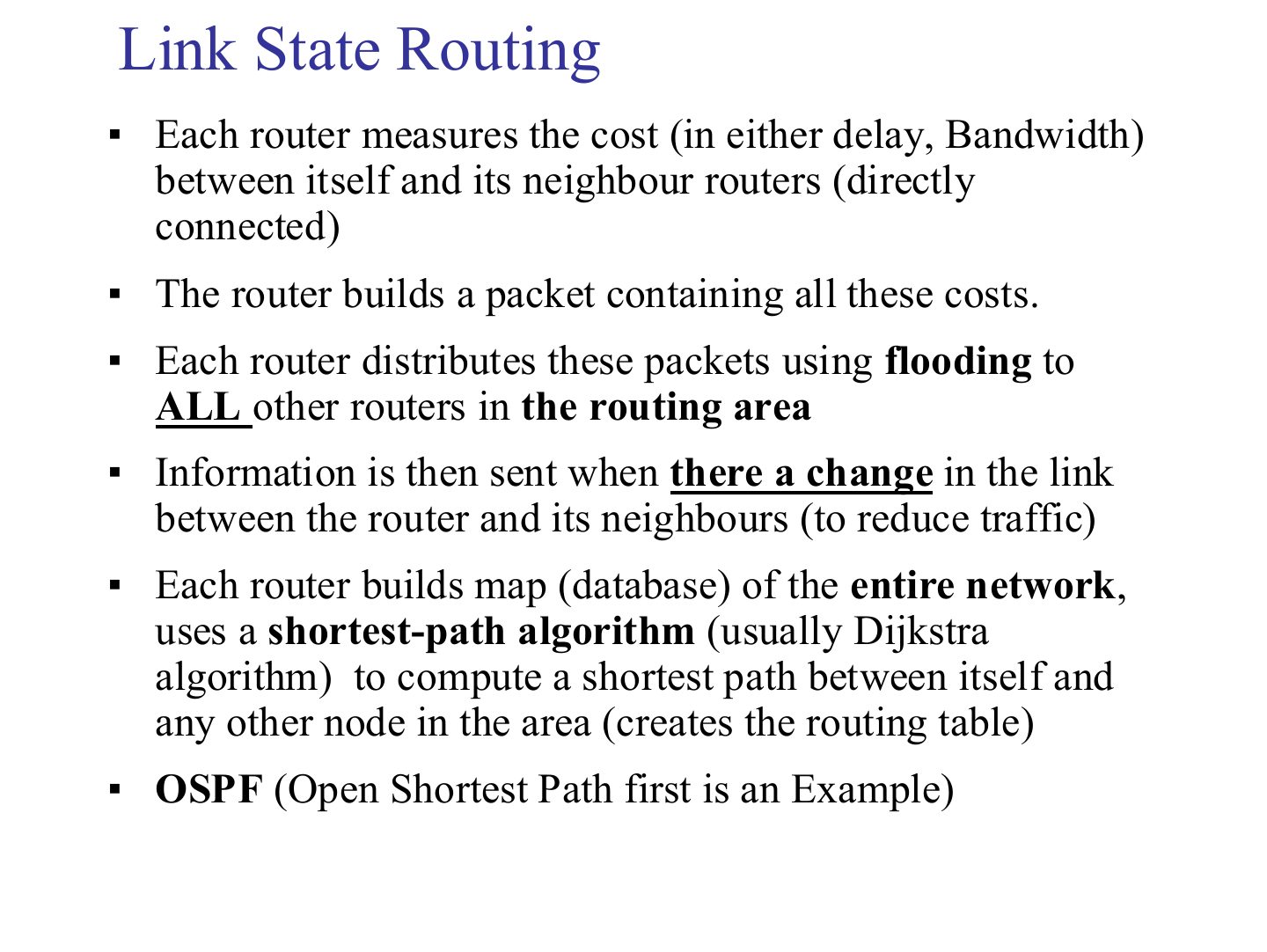
- 30 Link State Routing
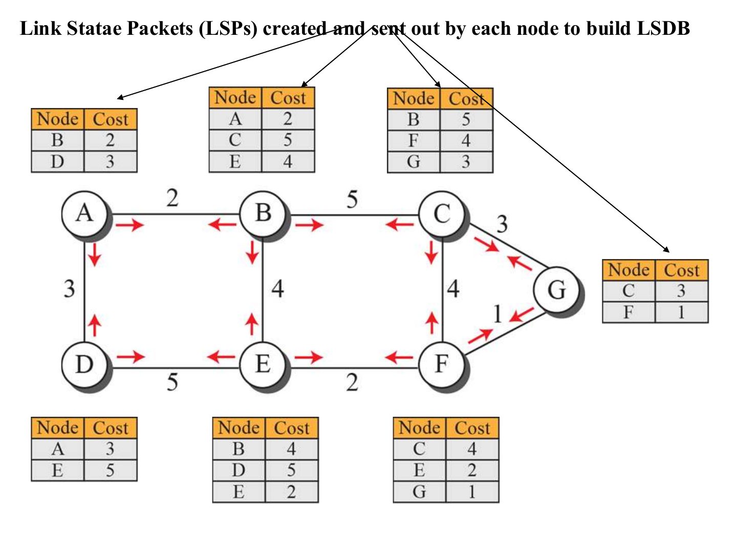
- 31 Link-state packets (LSPs) build the LSDB
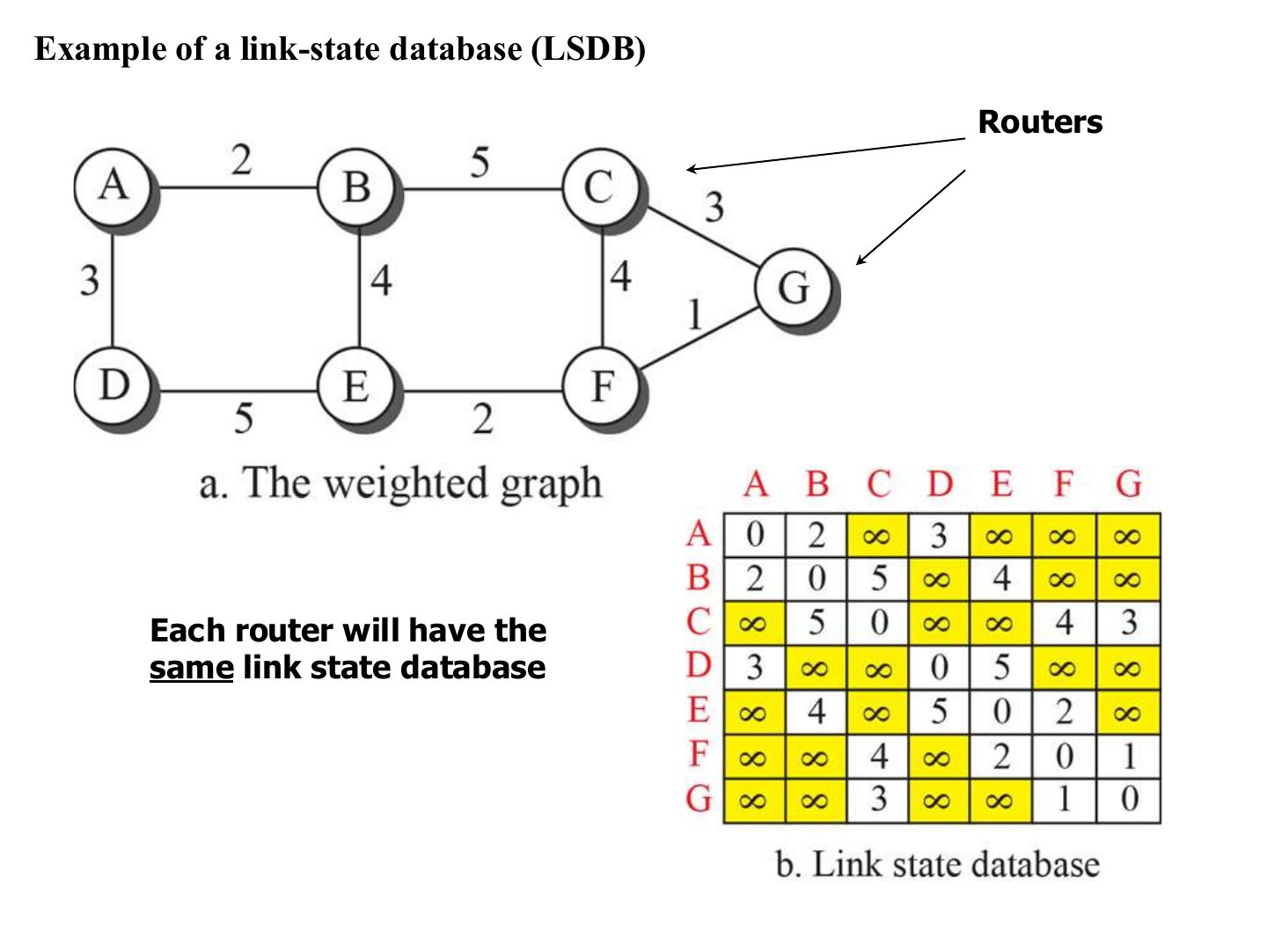
- 32 Example of a link-state database (LSDB)
- 33 Comparison between distance vector and link state
- 34 Autonomous systems (AS)
- 35 A sample internet with four ASs
- 36 Popular routing protocols
Network Layer: Routing of Packets
Notes
Routing vs. forwarding → graph model → static vs. dynamic → table tricks (network-specific, host-specific, default) → forwarding with masks → DV vs. LS → AS, IGP and BGP.
Chapter 8: Outline
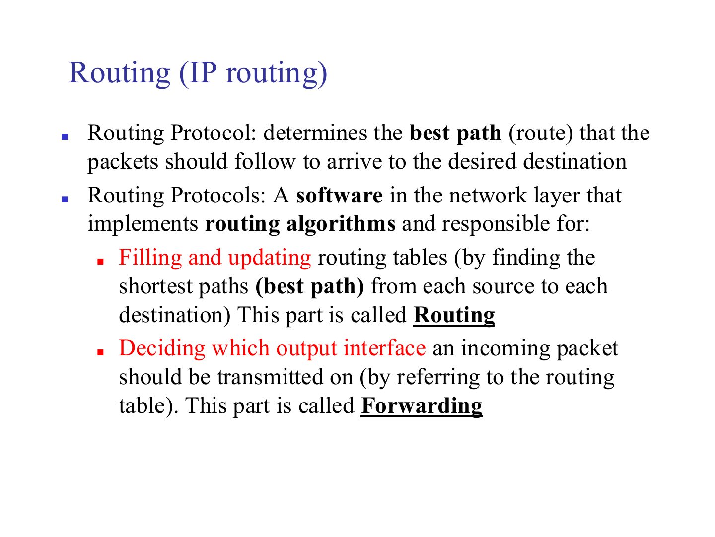
Routing (IP routing)
Notes
Routing protocol = software that FILLS the routing table (routing) and uses it to pick the output interface (forwarding).
Seen again Ch 7, slide 5: Routing vs. forwarding
Exam angle
8-1 INTRODUCTION
Notes
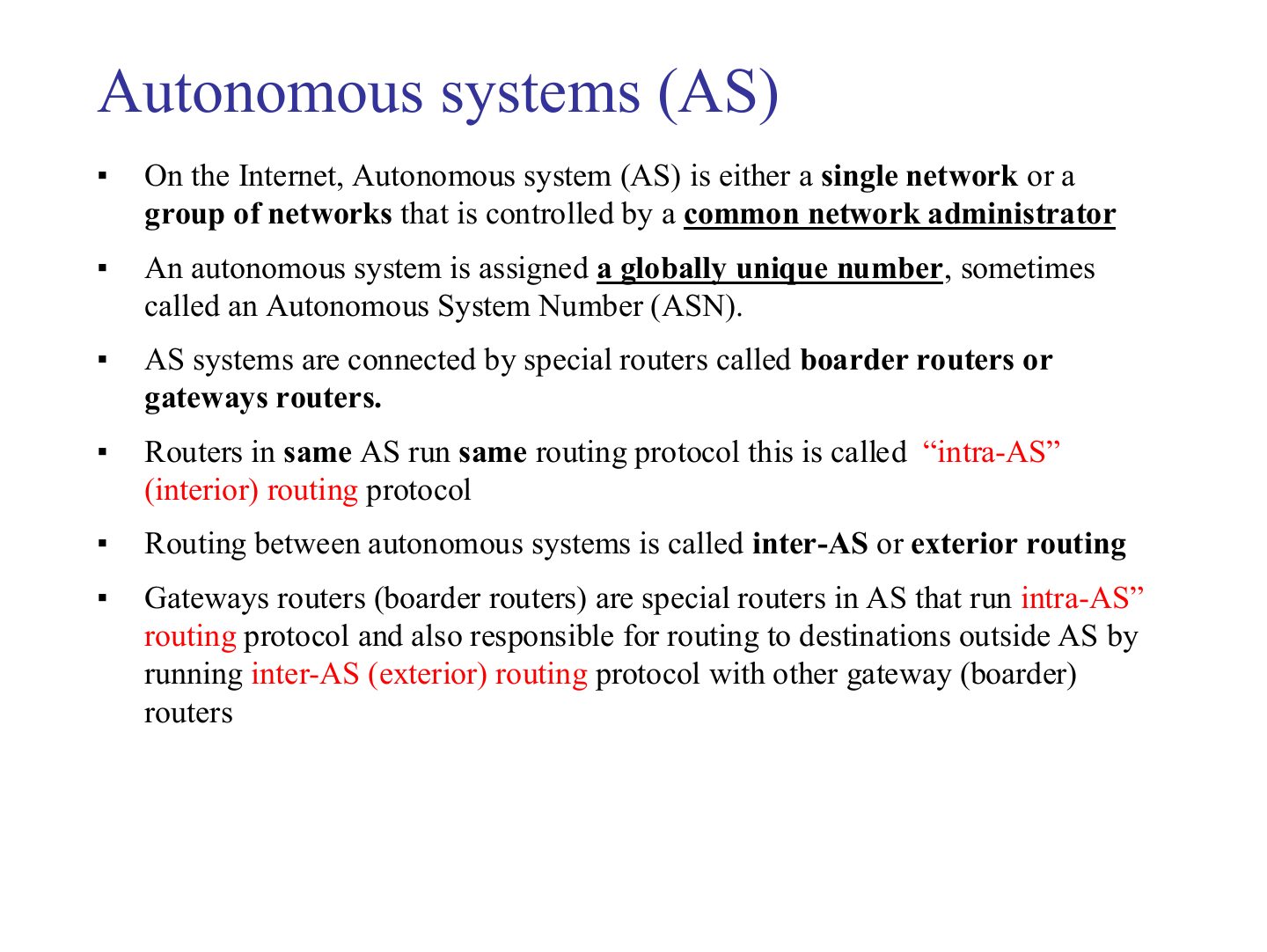
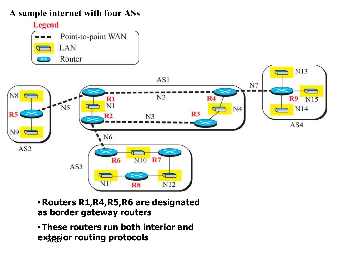
The Internet is too big for one algorithm, so routing is hierarchical (inside each AS, then between ASs: slide 34).
8.1.1 General Idea
Notes
Hosts just send to their default router; only routers need real forwarding tables.
An Internet as a Graph
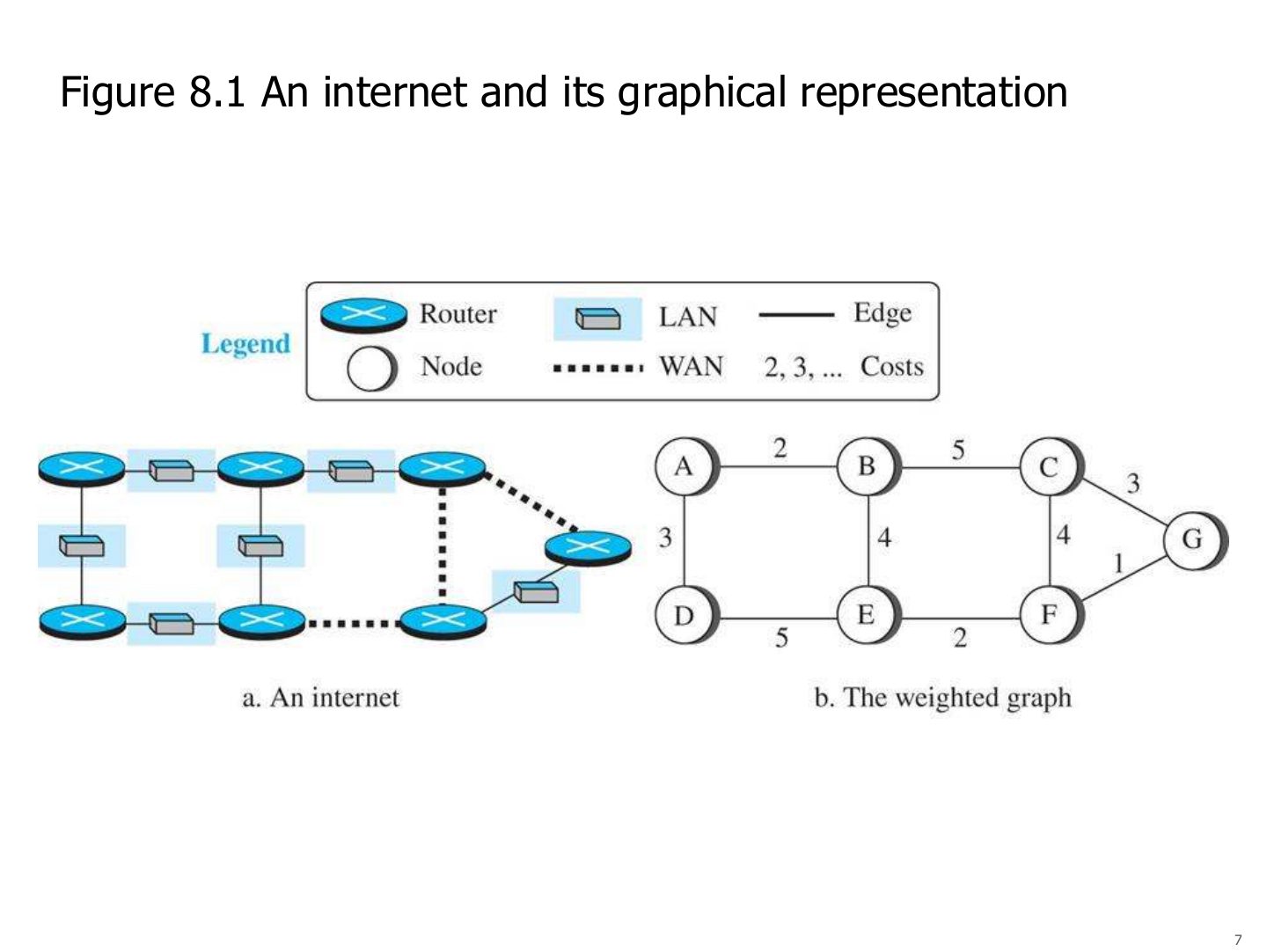
An internet and its graphical representation (Figure 8.1)
Notes
This A–G graph is reused in every DV and LS example below.
Graph representation of a network
Notes
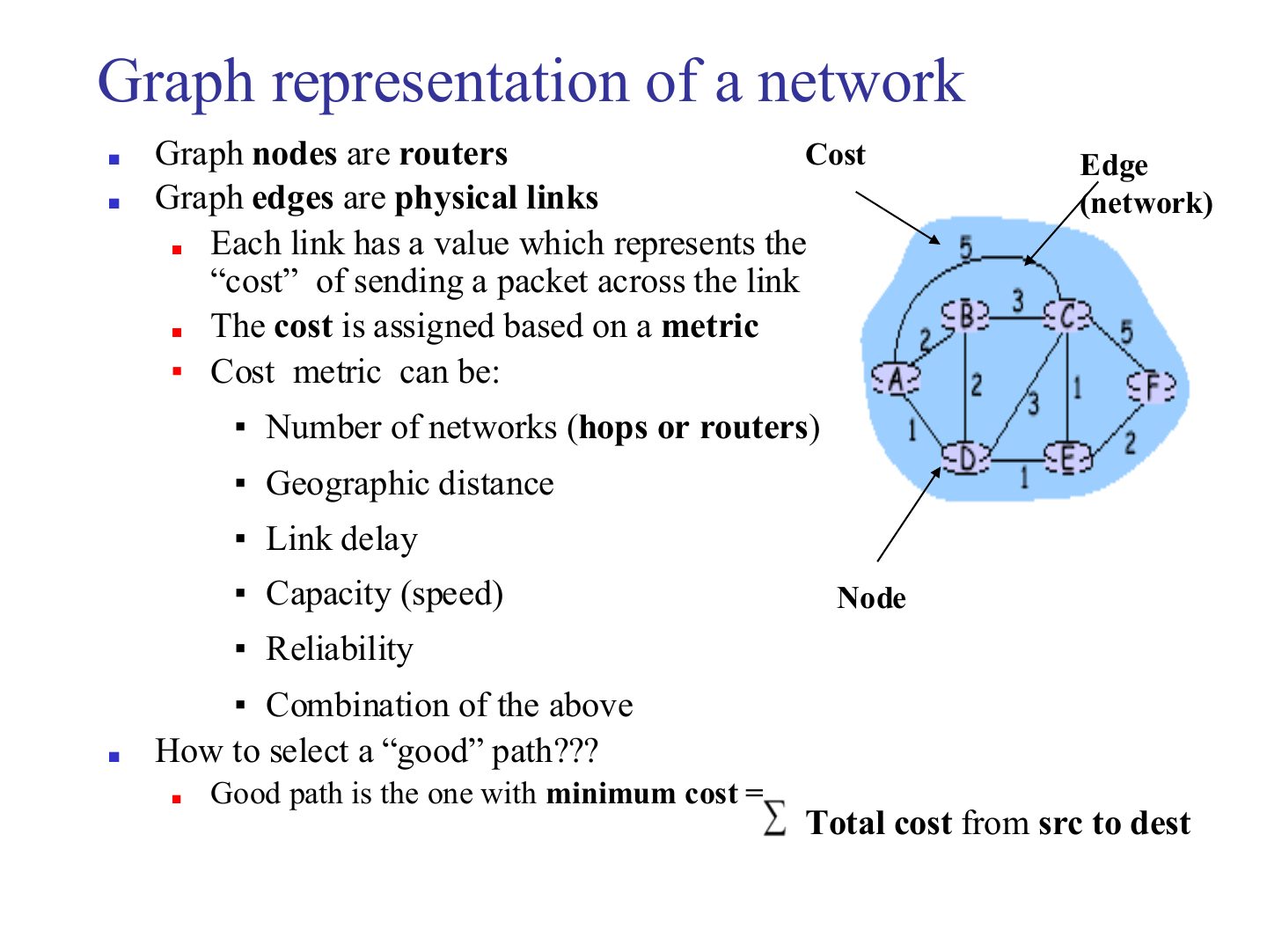
Best path = minimum TOTAL cost from source to destination.
Exam angle
Which is NOT listed as a possible link cost metric?
Routing Algorithms Classifications
Notes
Trap Static routes do NOT update automatically after a failure.
Exam angle
Static routing updates automatically when a link fails.
Compare static and dynamic routing.
Compare with the model answer
Static: shortest paths are computed offline and entered manually by the administrator; they change slowly, can’t adapt to failures, and suit small networks. Dynamic: each router learns the network state by talking to its neighbours and fills its own table automatically, adapting to changes, at the cost of more router complexity.
Routing algorithm: dynamic route operation
Notes
Routing protocols on neighbouring routers swap updates to keep tables current.
How to reduce number of entries in the routing table?
Notes
Three ways to keep the table short or specific: network-specific, host-specific and default routes.
Host-specific versus network-specific method
Notes
Host-specific: one row per HOST (A, B, C, D via R1). Network-specific: one row for the whole network N2 → much smaller.
Exam angle
Listing one entry for a whole destination network instead of each host is:
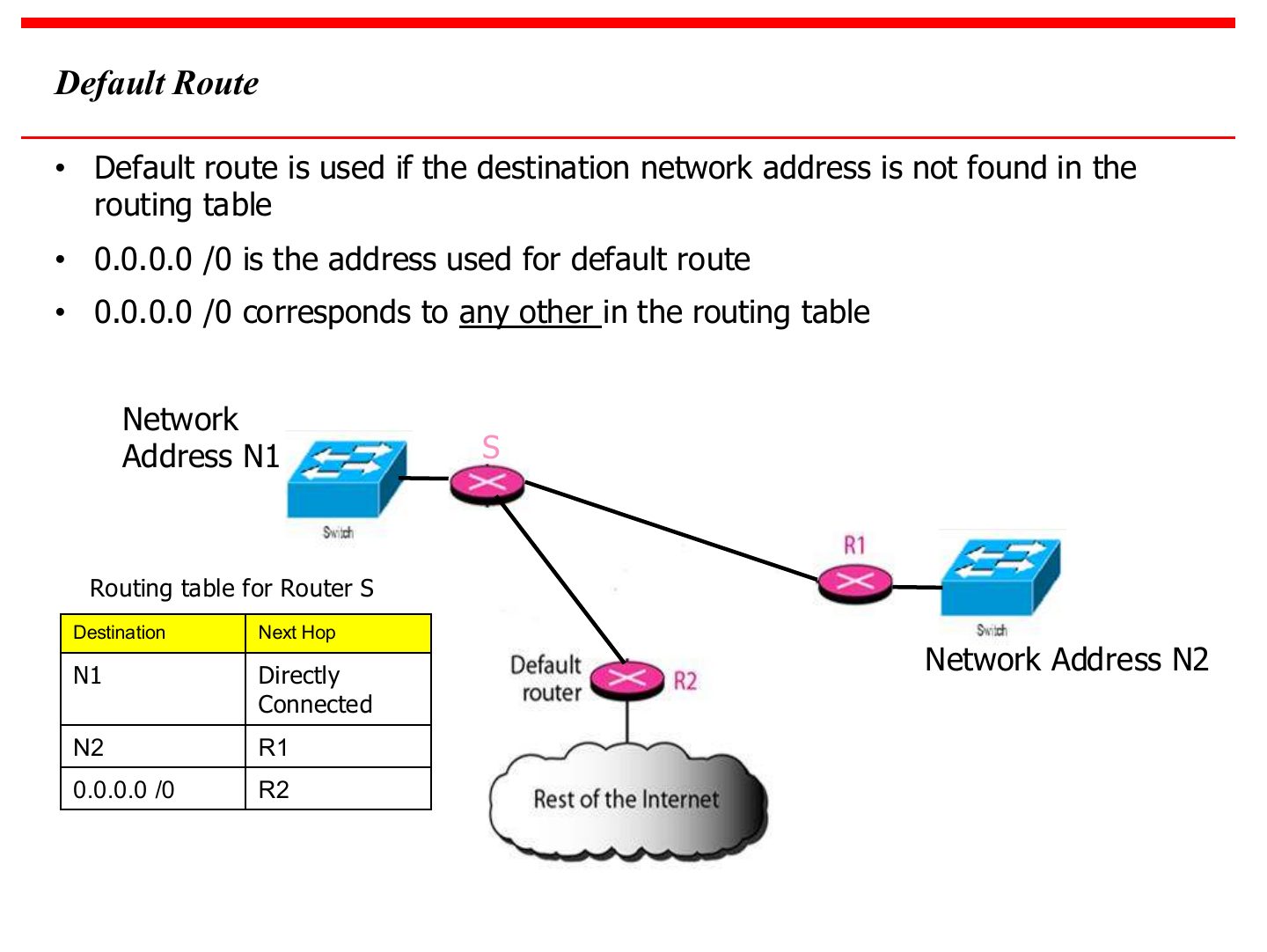
Default Route
Notes
Default route 0.0.0.0/0 = “everything else”: here, go to R2 (towards the Internet).
Exam angle
The default route is written as:
Forwarding of IP packets
Destination Address Forwarding
Classful addressing routing table
Notes
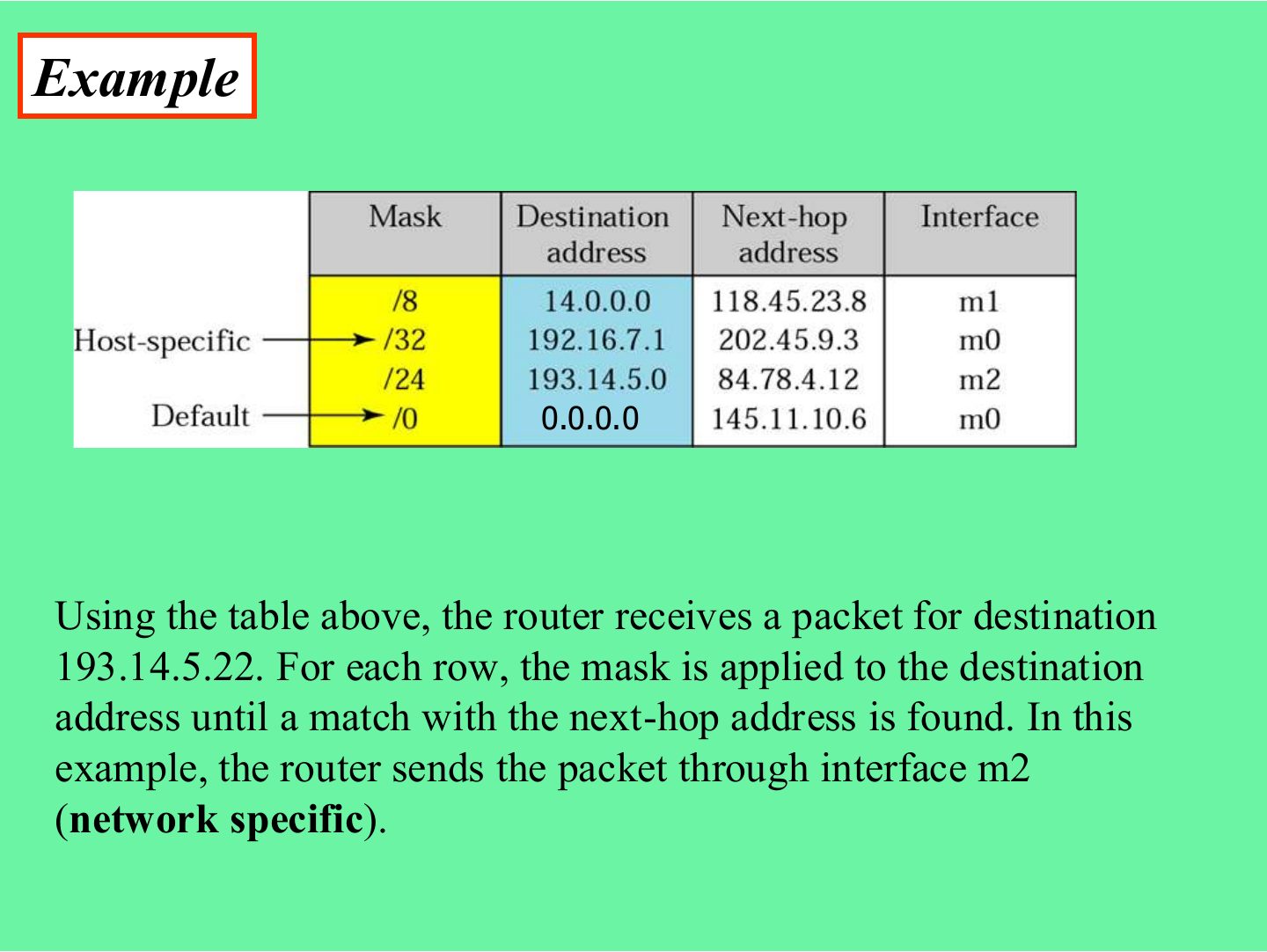
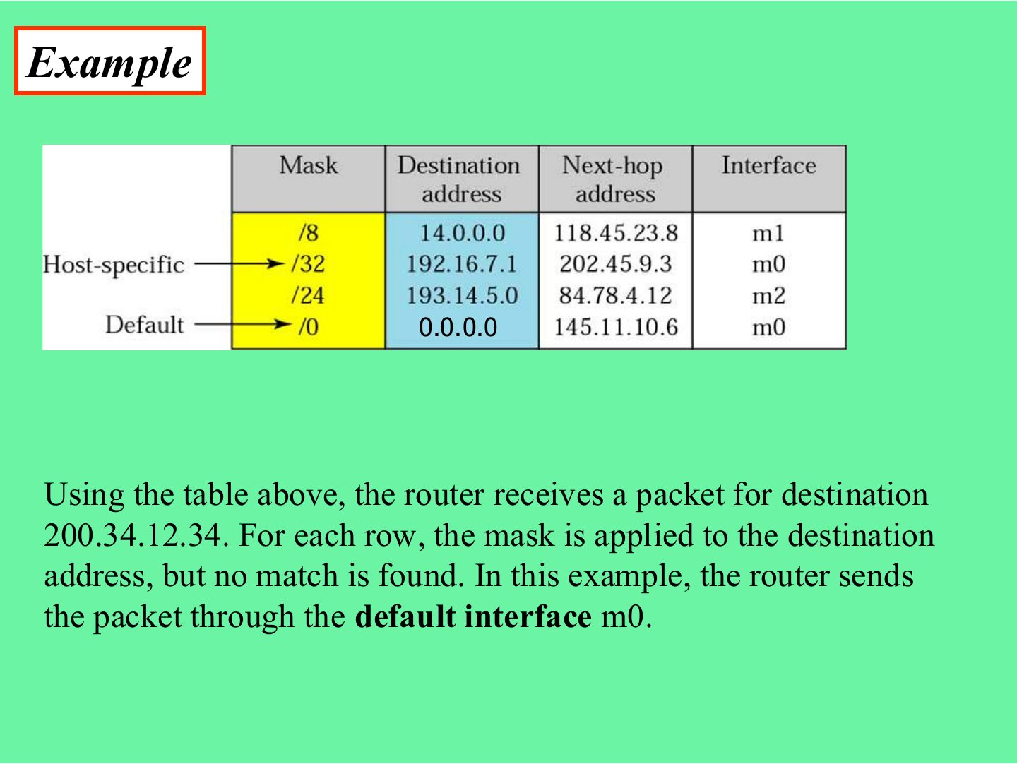
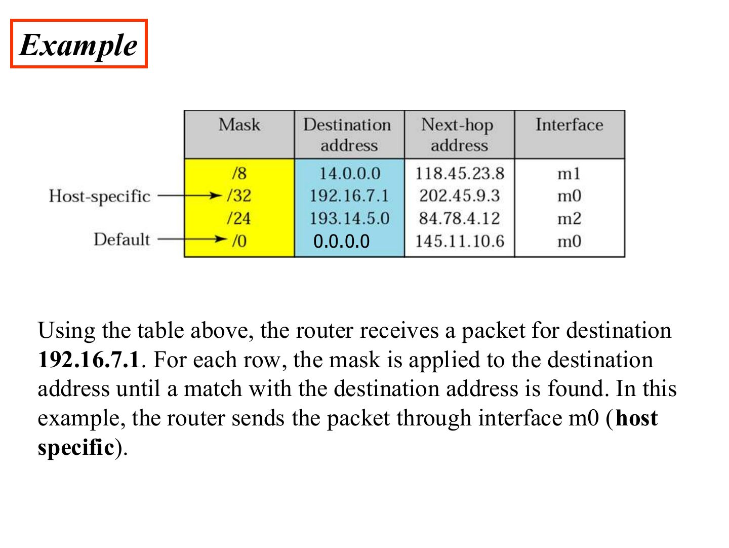
Try each mask on the destination; the first row that matches wins. /32 = a host-specific row, /0 = default.
Example
Exam angle
Using the table, a packet for 14.5.6.7 leaves through:
- /8 → 14.0.0.0 matches → m1.
Example
Example
Exam angle
A /32 row in a routing table is a:
Example: router R1’s networks
Notes
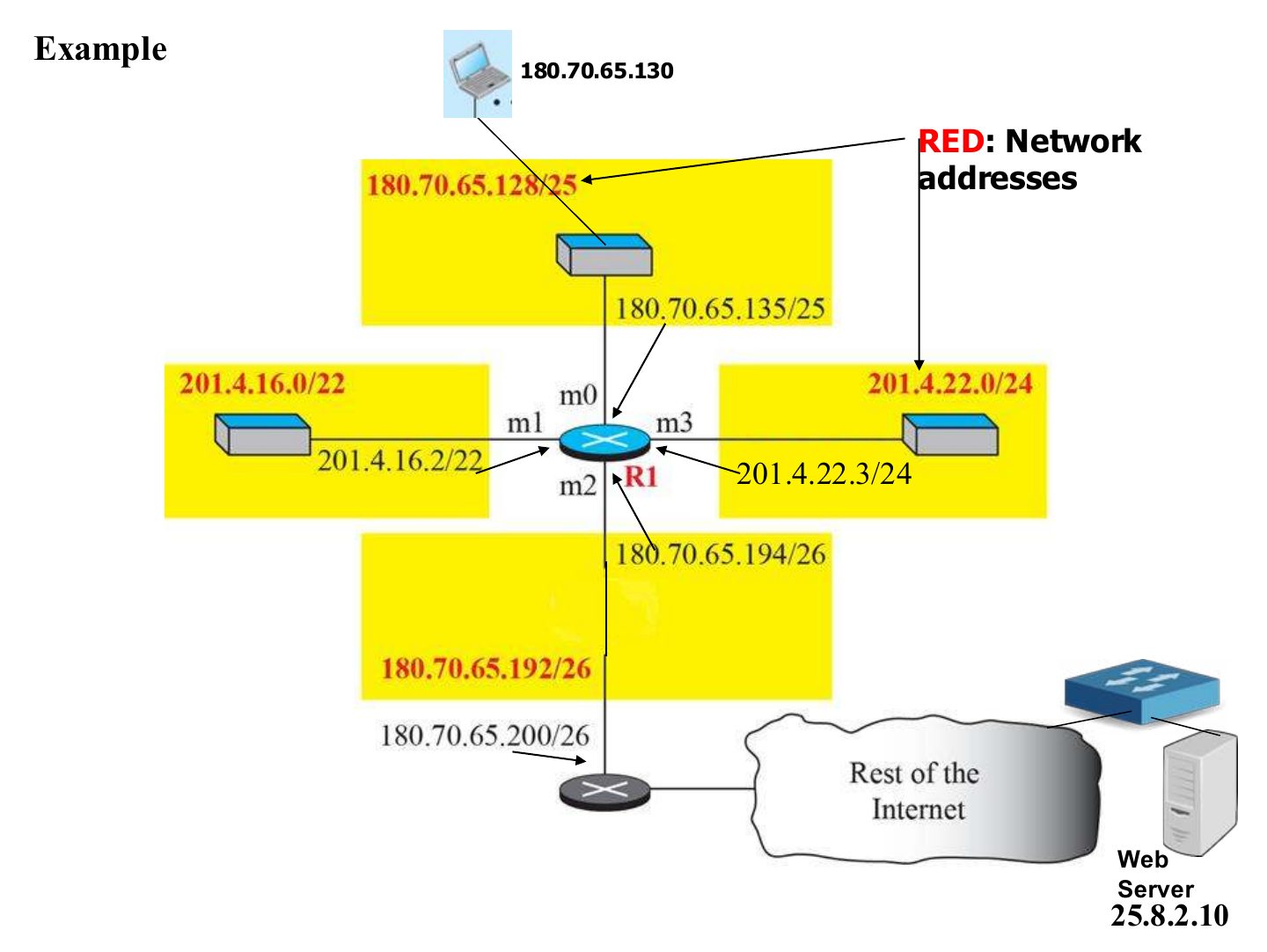
Four attached networks plus a path to the rest of the Internet through 180.70.65.200.
Forwarding table for router R1
Notes
Rows are sorted from the LONGEST mask (/26) to the shortest (/22), with the default (/0) last. Longest match wins.
Memory trick Longest prefix first, default last.
Show the forwarding process if a packet arrives at R1 with the destination address 180.70.65.130.
Notes
/26 gives .128 (the row wants .192) → no. /25 gives .128 → match → m0.
Exam angle
Using R1’s table, a packet for 201.4.22.35 leaves through:
- /24 → 201.4.22.0 matches.
Using R1’s table, a packet for 201.4.18.7 leaves through:
- /22 → 201.4.16.0 matches (16–19).
Show the forwarding process if a packet arrives at R1 with the destination address 25.8.2.10.
Exam angle
R1 receives a packet for 25.8.2.10. Walk through the forwarding steps.
Compare with the model answer
Apply /26 → 25.8.2.0 (no match), /25 → 25.8.2.0 (no), /24 → 25.8.2.0 (no), /22 → 25.8.0.0 (no). Nothing matches, so the default row 0.0.0.0/0 is used: send to next hop 180.70.65.200 through interface m2.
Shortest Path Routing
Exam angle
Link-state routing uses which algorithm?
Distance-vector routing is based on:
Distance Vector (DV) Routing
Notes
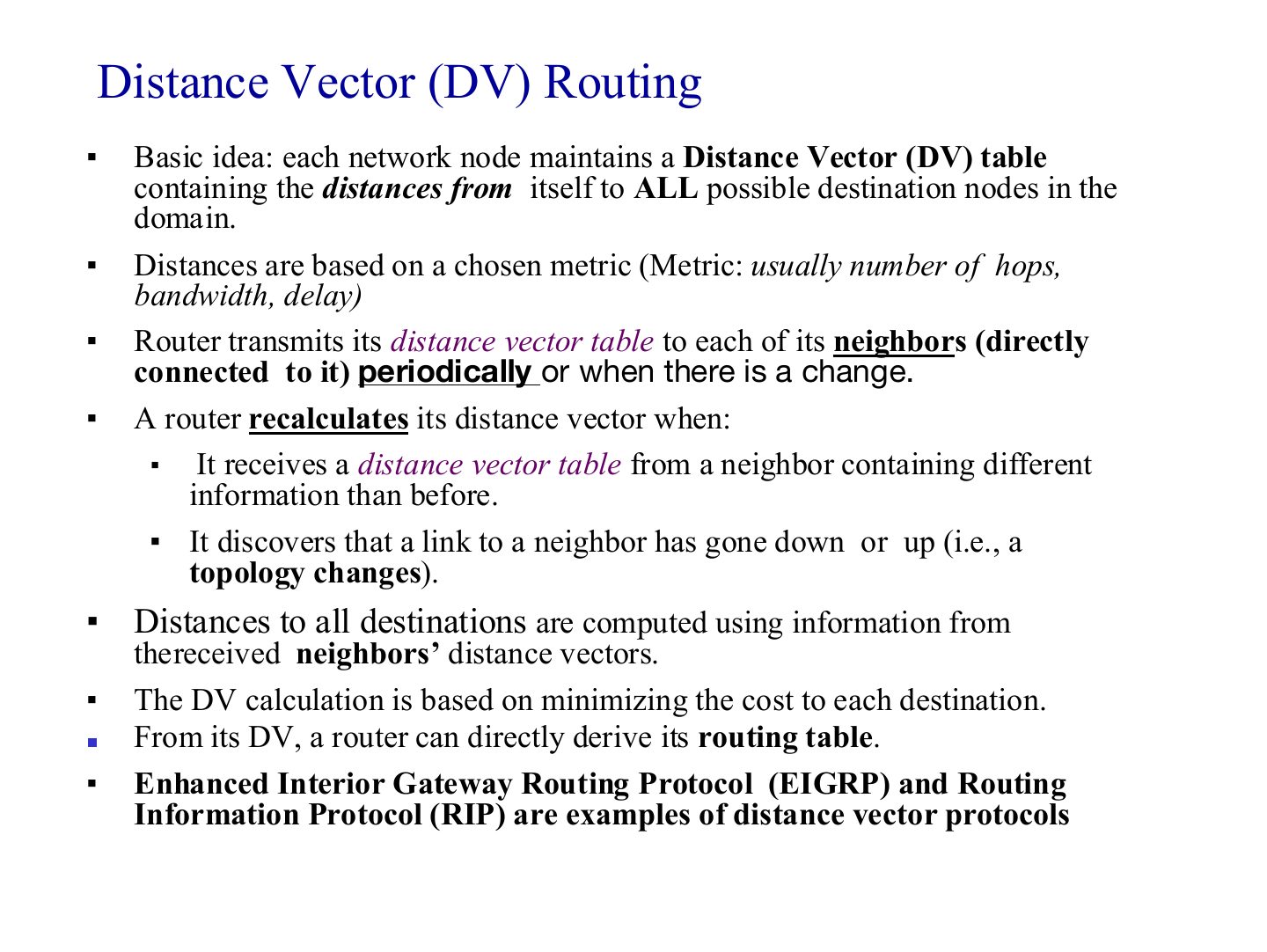
Each router keeps distances to ALL destinations and sends that whole vector to its NEIGHBOURS, periodically or on change.
Memory trick DV = “tell your NEIGHBOURS about the WHOLE world”. LS = “tell the WHOLE world about your NEIGHBOURS”.
Exam angle
Which is a distance-vector protocol?
The first-round distance vectors
Notes
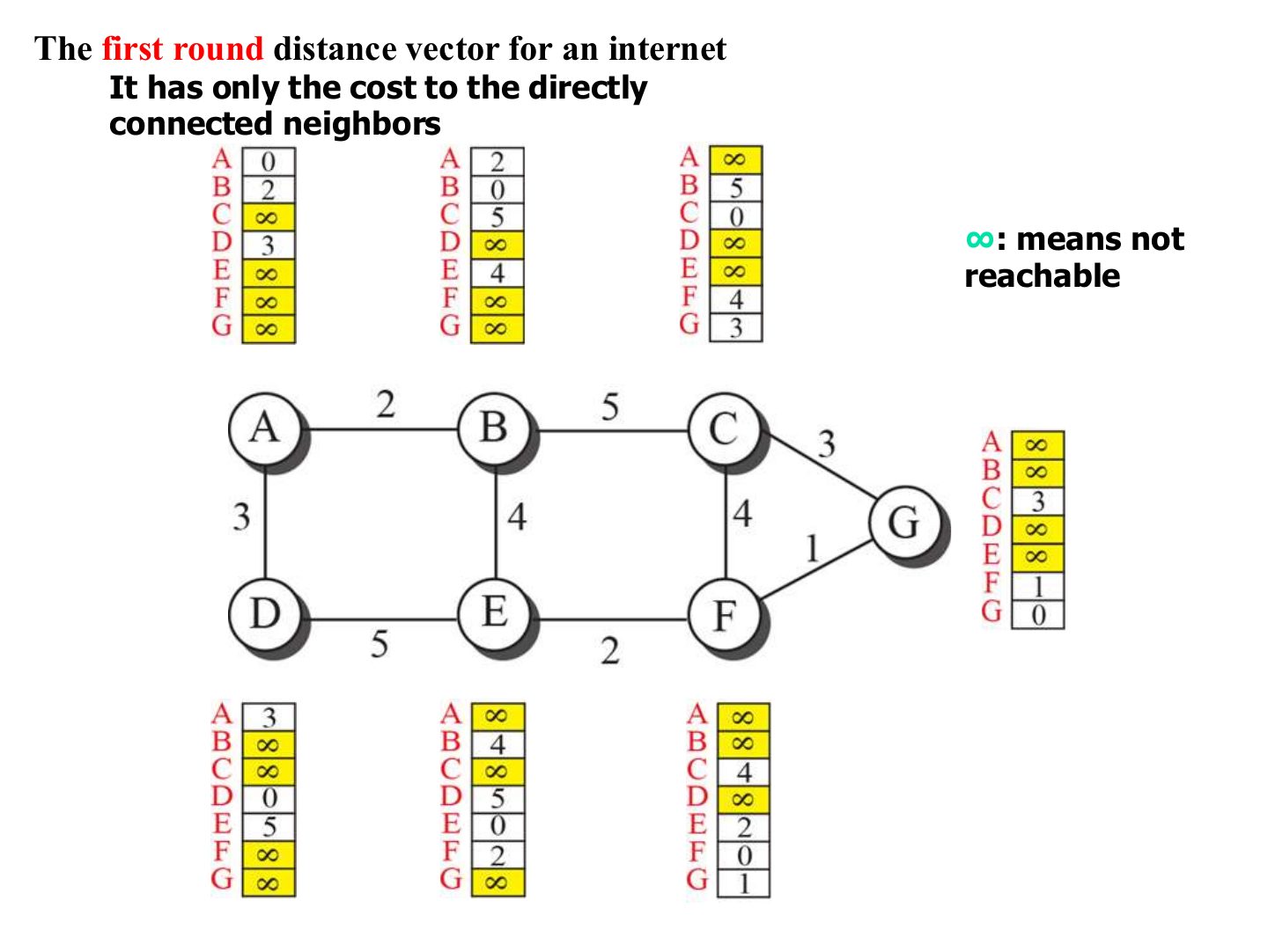
Round 1: only neighbour costs, everything else ∞.
Updating distance vectors (node B)
Notes
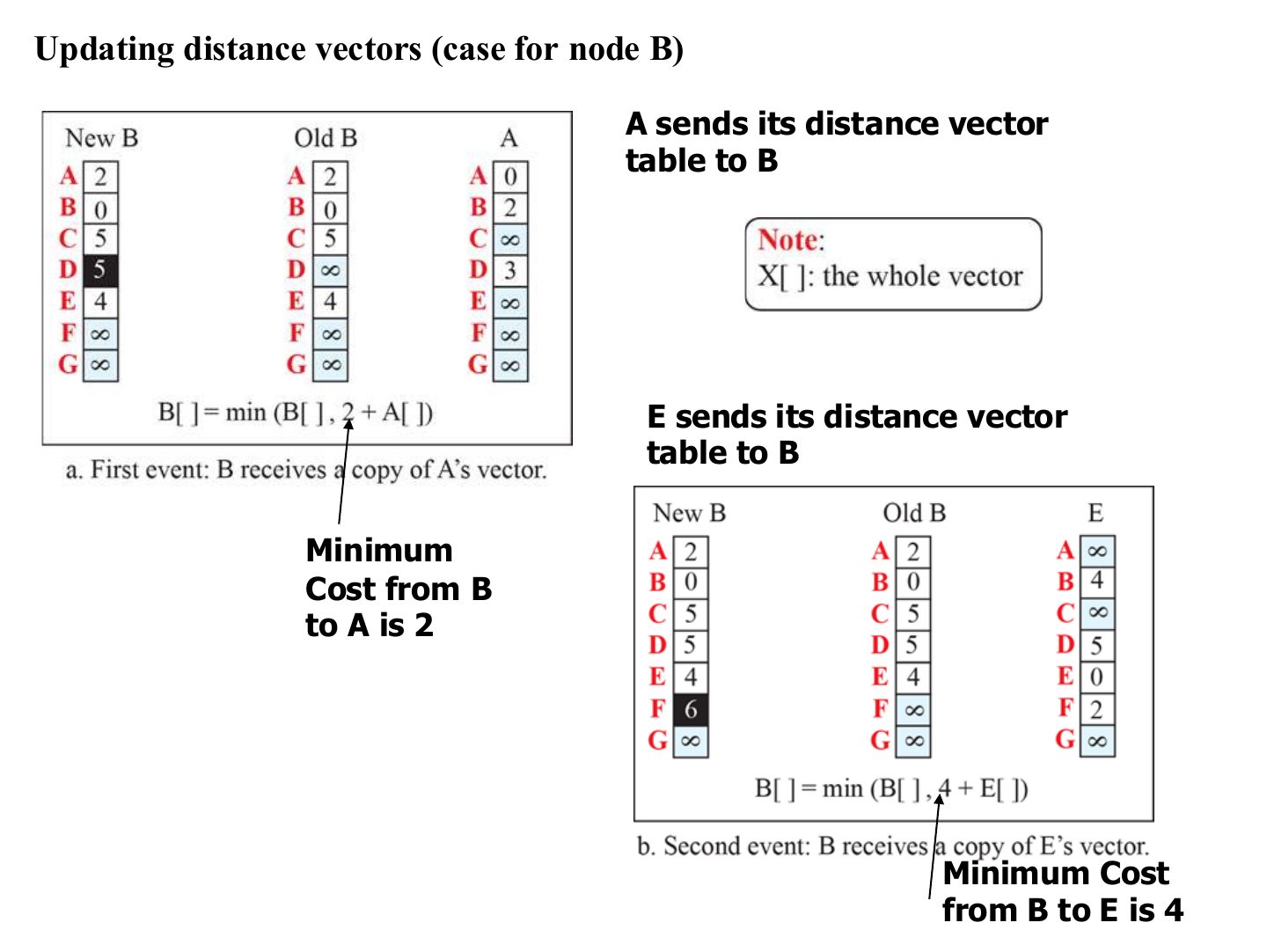
Bellman-Ford: new cost to X = min(old cost, cost to neighbour + neighbour’s cost to X).
Exam angle
B–A costs 2 and A’s cost to D is 3. B currently has D at ∞. After A’s update, B’s cost to D is:
- min(∞, 2 + 3).
State the Bellman-Ford update rule used in distance-vector routing.
Compare with the model answer
Dx(y) = min over neighbours v of [c(x, v) + Dv(y)]: the cost from x to y is the cheapest of “cost to a neighbour plus that neighbour’s advertised cost to y”, compared with the current value.
The distance vector corresponding to a tree
Notes
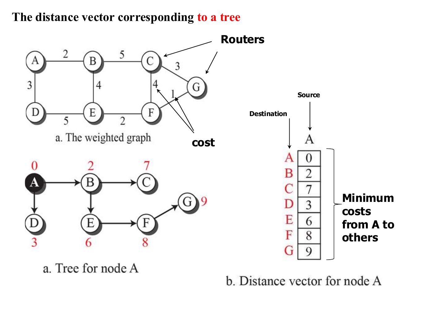
A’s final vector: B 2, C 7, D 3, E 6, F 8, G 9.
Exam angle
In the slide’s graph, the least cost from A to G is:
- A–B–E–F–G = 2 + 4 + 2 + 1 = 9.
Least-cost trees for nodes for the previous network
Notes
Every node ends up with its own least-cost tree.
Link State Routing
Notes
Every router builds the same map (LSDB) and runs Dijkstra itself. OSPF is link state.
Exam angle
Which is a link-state protocol?
In link-state routing, each router sends its link costs to its neighbours only.
- It floods them to all routers in the area.
Link-state packets (LSPs) build the LSDB
Notes
An LSP = “my neighbours and their costs”.
Example of a link-state database (LSDB)
Notes
All routers share the same LSDB (the whole map) but each computes its own tree.
Comparison between distance vector and link state
Notes
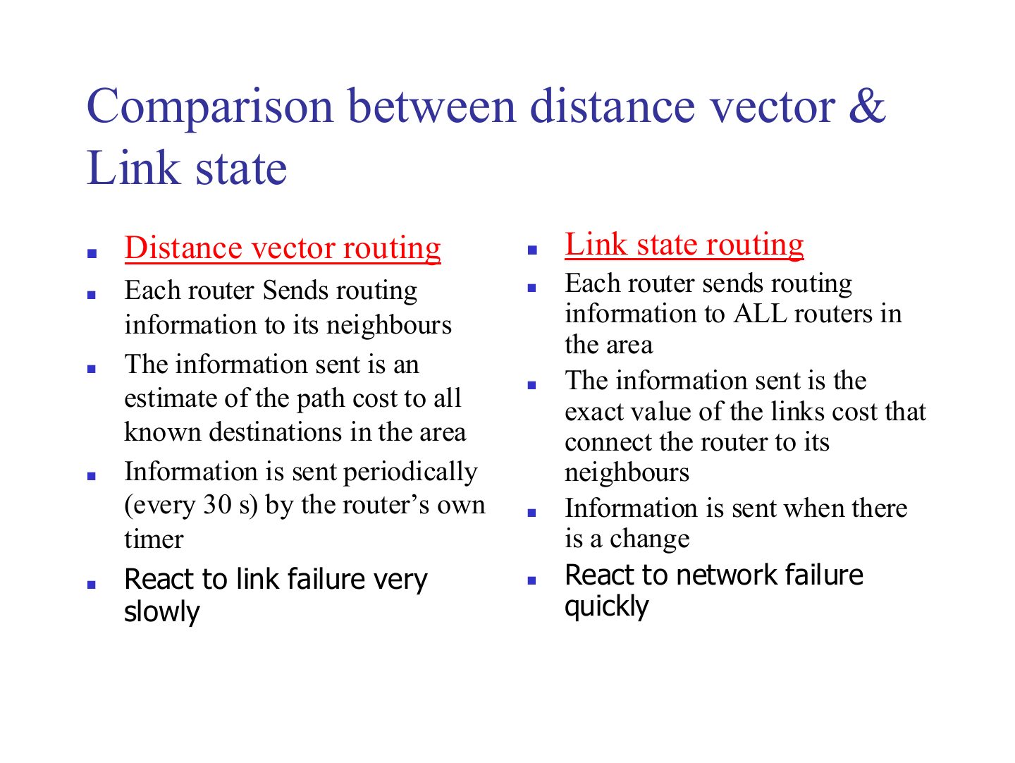
DV: to neighbours, estimates of everything, periodic, slow to react. LS: to all, exact neighbour costs, on change, fast.
Exam angle
Compare distance-vector and link-state routing (who receives updates, what is sent, when, and reaction to failure).
Compare with the model answer
Distance vector: sends to neighbours only; sends its estimated cost to every known destination; periodically (e.g. every 30 s); reacts to failures slowly. Link state: floods to all routers in the area; sends the exact cost of its own links to its neighbours; only when something changes; reacts to failures quickly.
Which reacts faster to a link failure?
Autonomous systems (AS)
Exam angle
Routing between autonomous systems is called:
A sample internet with four ASs
Popular routing protocols
Notes
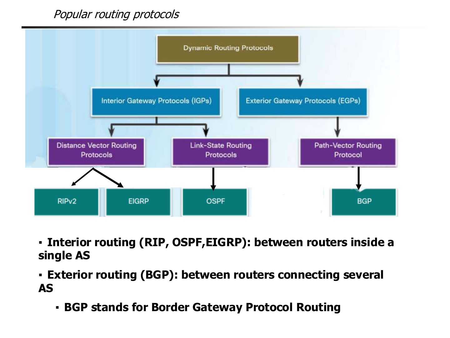
Interior: RIP, EIGRP (distance vector), OSPF (link state). Exterior: BGP (path vector).
Memory trick Only one exterior protocol to know: BGP, the B is for Border.
Exam angle
Which protocol routes between autonomous systems?
EIGRP is a: